Section 5 Normalization
Correct technical biases and prepare your datasets for further analyses:
- Basic transformations (log transformation, scaling to unit variance, quantile normalization)
- Normalizations specific of certain data types (for count data like RNA-seq or for compositional data like metagenomics)
- Normalization for the correction of an explicit batch effect
- All normalization methods come with diagnostic plots.
5.1 Standard transformation
5.1.1 Logarithm transformation
5.1.1.1 Interpretation


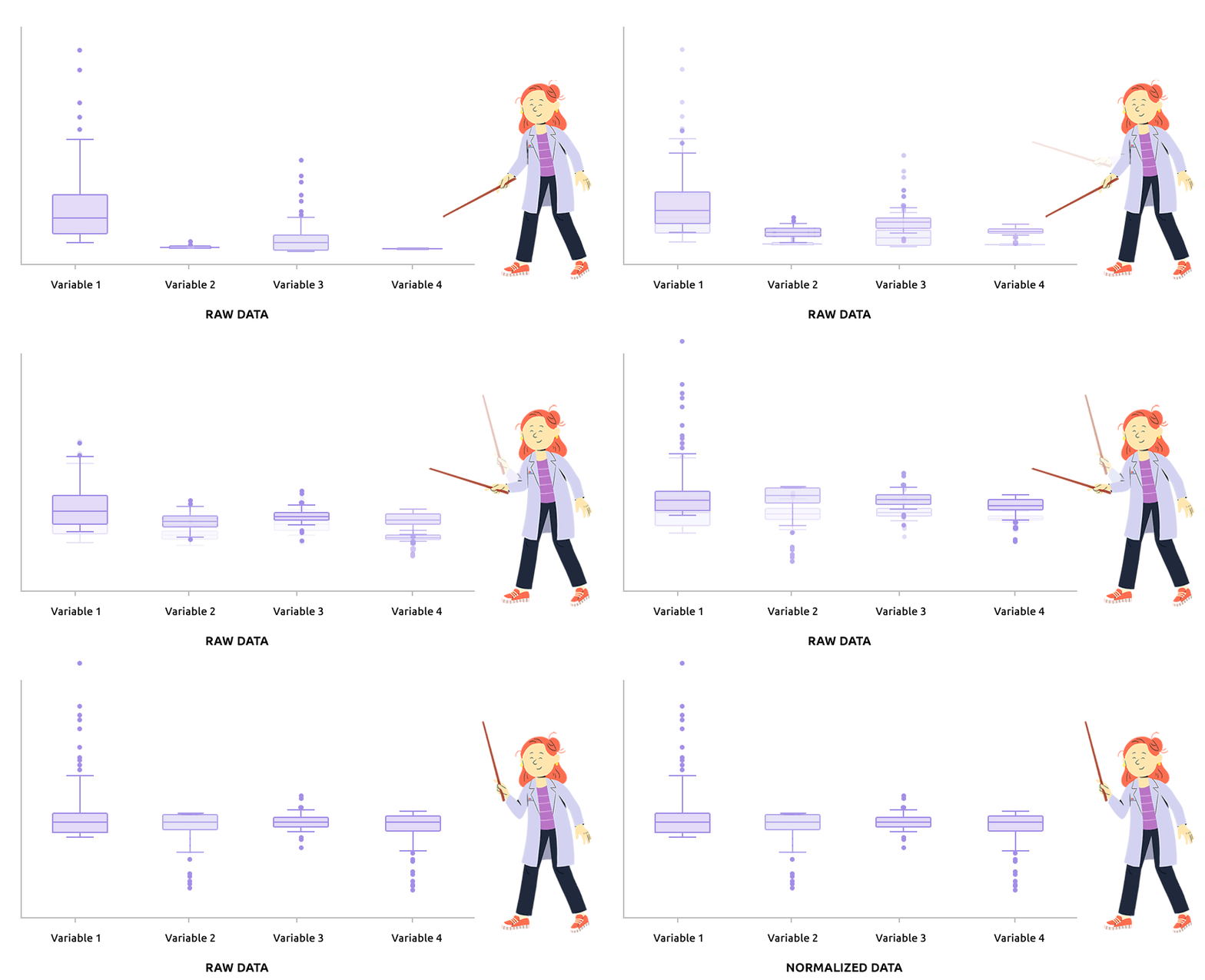
Logarithm transformation aims at making variable distributions closer to the Gaussian distribution. This is a requirement for parametric tests (ANOVA, Student, …) and it is advised for exploratory analysis. In particular, it is usual to use these transformations on microarray data for all subsequent analyses or on TMM / TMMwsp normalized RNA-seq data for subsequent exploratory analyses (PCA, clustering, …).
On the before/after boxplot, check that the variable distributions are symmetric, with only a few outliers.

For RNA-seq data, check the corresponding menu that provides an option to combine normalization and log-transformation.
5.2 Quantile normalization
5.2.1 Interpretation

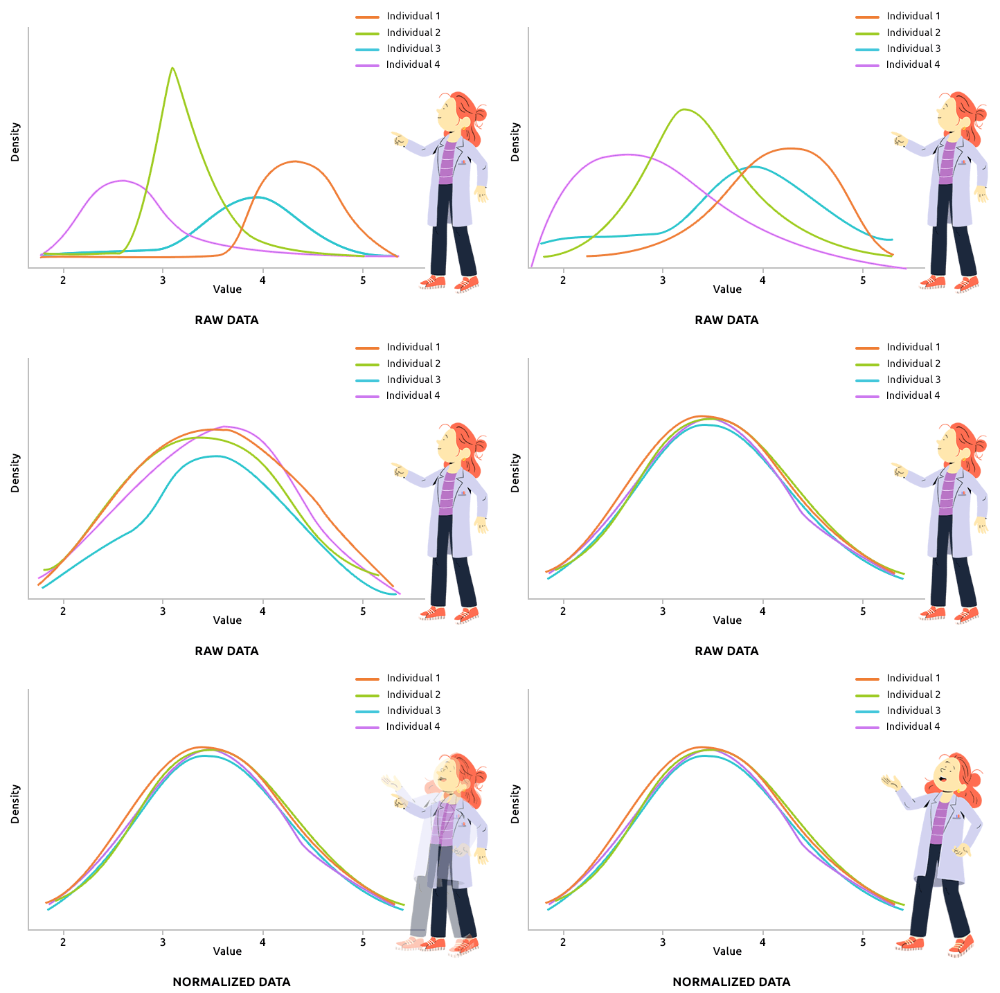
Quantile normalization aims at aligning the distributions of all individuals (over all variable values). This type of normalization is usually advised to correct technical biases in some experiments that produce a large number of continuous measurements (like microarray data, after they have been log2-transformed, for instance). Check that all density plots are well aligned after quantile normalization.
5.3 RNA-seq (and other count) data
5.3.1 Interpretation
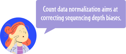
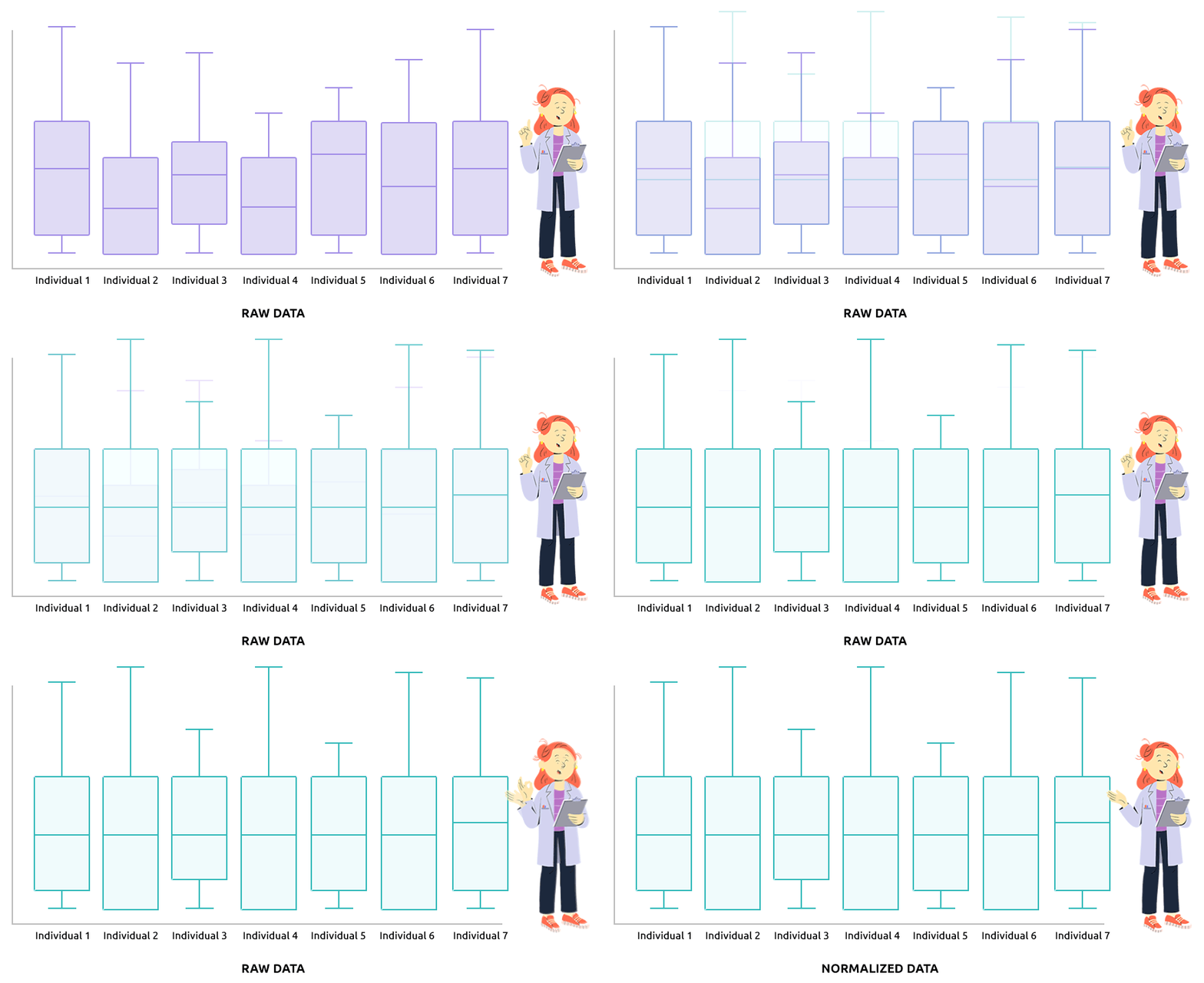
Two different types of normalization are implemented: TMM (which is advised
in most cases) and TMMwsp, both as implemented in the R package
edgeR). These normalizations aim at correcting the sequencing depth bias
and making counts comparable between individuals. TMMwsp is to be preferred over
TMM when the number of zeros in your data is large.
Check that the boxplots are similar after normalization.

These normalizations are designed for count data. If your RNA-seq data are already normalized, you must not use them (and the results of your tests might be incorrect because tests for count data use both raw and normalized data).
If your data are already log-transformed, you can undo this log-transformation and perform the TMM or TMMwsp normalization. Log-transformed RNA-seq counts have to be used for exploratory analyses (PCA, clustering, …) but should not be used for tests.
5.3.2 Default parameters
Used function and default parameters:
The normalisation for count data consists in three steps, according to those who have been chosen by the user:
filter: remove the values inferior or equal to a certain value,
TMM:
edgeR::calcNormFactorswith optionmethod = 'TMM',log(cpm(x) + prior.count) : it’s a log transformation on cpm values computed this way :
edgeR::cpm(y = df, lib.size = lib.size).
5.4 Compositional data
5.4.1 Interpretation

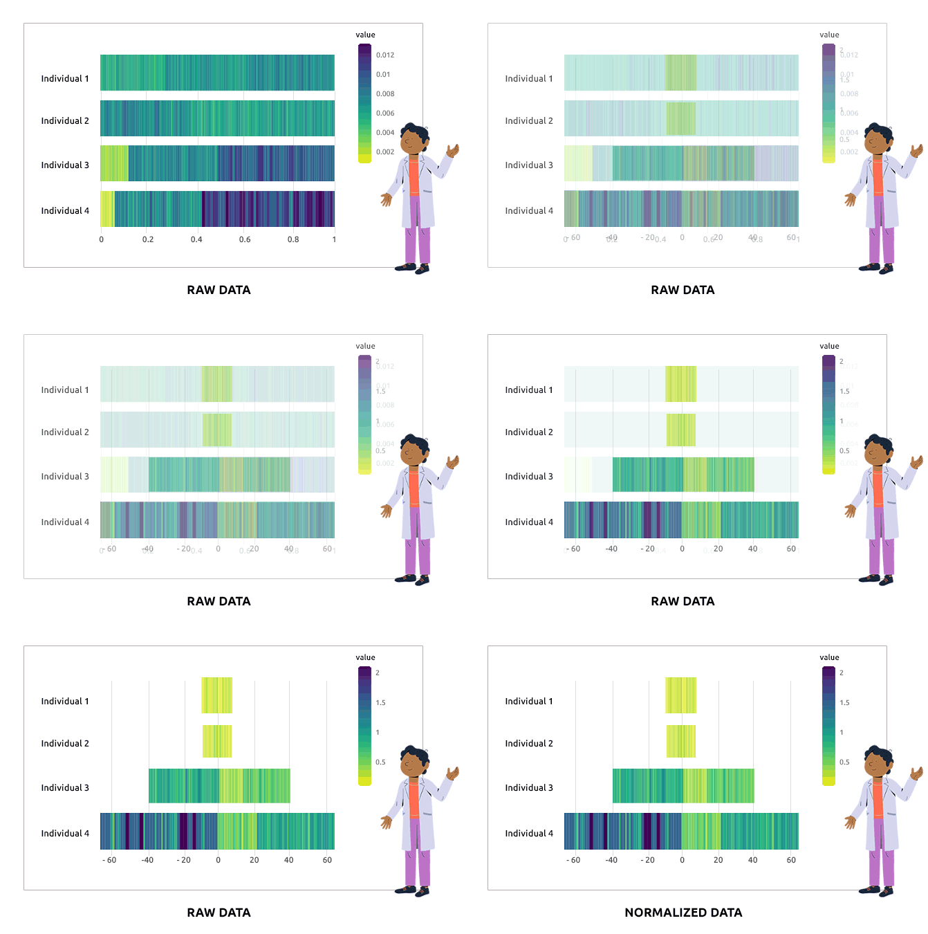
Compositional data are data for which the sum of all variable values for a given individual is always the same (e.g., percentages are compositional data because they sum to 1). Such data are not adequate for a direct use in statistical analyses. We propose different types of transformations that correct this problem. Barplots are used to represent the value of each variable in each individual. It is expected that bars corresponding to individuals have varying heights after the transformation.
5.4.2 Default parameters
Used function and default parameters:
If the dataset is seen as count data, the normalization consists in three steps:
If the dataset is seen as compositional data, the normalization consists in three steps:
offset: add a value to all cells in the dataset (
df + offset),filter: remove the values inferior or equal to a certain value,
normalization: one of the following methods, chosen by the user:
CLR:
compositions::clrwith the default parameters,ILR:
compositions::ilrwith the default parameters,CSS:
metagenomeSeq::cumNormStatFast, with the default parameters.
5.5 Metagenomic data
5.5.1 Interpretation
Metagenomic data can be considered as count data (like RNA-seq) or as compositional data. Both situations are handled with different normalization methods (similar to the ones described in the corresponding tabs).

When considering metagenomic data as count data, TMMwsp normalization might be
a better choice than TMM because it accounts for the excess of zeros that
metagenomic data usually have.
Be careful to check if your metagenomic data are already log-transformed or not
before you choose a normalization.
5.5.2 Default parameters
Used function and default parameters:
The normalisation for metagenomics data uses these function, depending on the kind of normalization done:
For CLR normalization:
compositions::clrwith the default parameters,For ILR normalization:
compositions::ilrwith the default parameters.
5.6 Correcting batch effect with ComBat
5.6.1 Interpretation

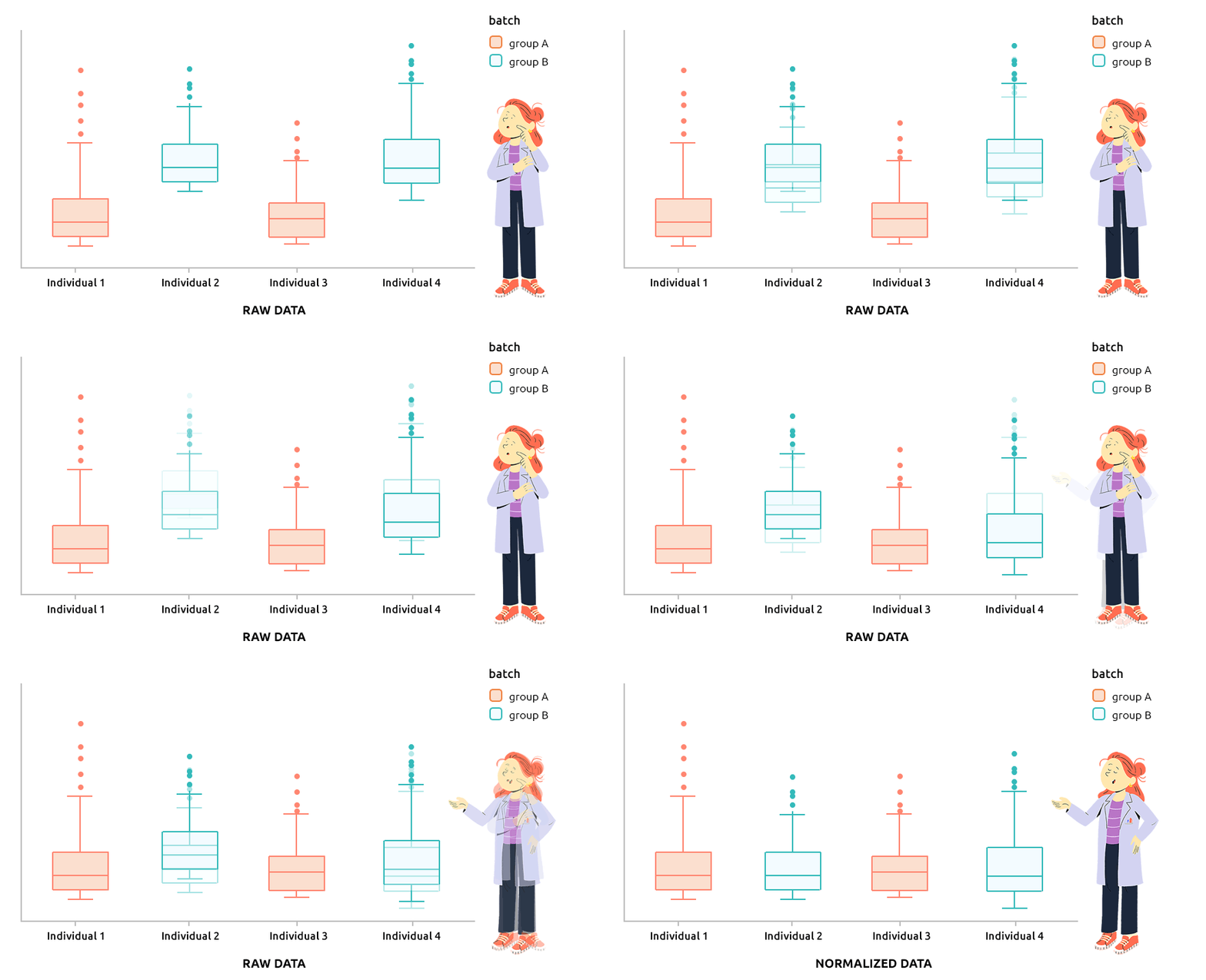
ComBat approach is the approach implemented in the R package sva and is designed to correct explicit batch effect (described by a factor that must be provided with the dataset to normalize). It can be applied to continuous data (like microarray data) or to count data (before TMM or TMMwsp normalization).
