Section 16 Case study: Breast cancer
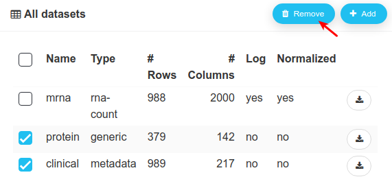
This case study focuses on breast cancer, trying to link omics data to cancer subtypes. There are four breast cancer subtypes that somewhat represent sub-diseases, with different biological mechanisms. Their identification is particularly important when designing / selecting treatments. For this case study, we have mRNA and miRNA data on 988 individuals, as well as the associated subtypes. mRNA data is already normalized and is loaded in ASTERICS by default, whereas miRNA comes in the form of raw counts.
The data is available online (ASTERICS team 2021).
16.1 Setup
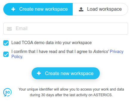
Let us open an empty session and load the TCGA demo data.
Since we will only use the mrna dataset, let us delete the other two.
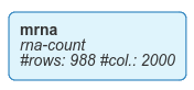
Here is mrna in the workspace:
Let us now import the subtypes (that can be found at https://doi.org/10.15454/YNMQUY). We click on the Add button:

Then, we select the file in our folder and set a generic nature.
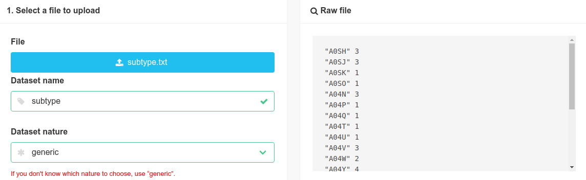
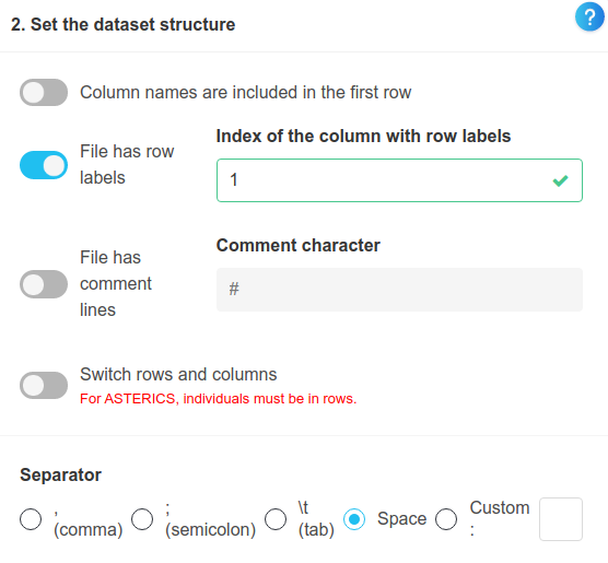
We then reflect in the settings the fact that a white space is used as a separator, and that there is no header in the file. After that, we import the dataset.
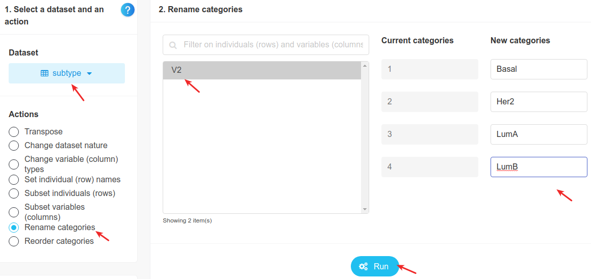
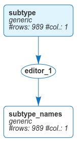
Once the dataset has been imported, we would like to give subtypes meaningful names instead of using integers from 1 to 4. We will do this in the edition module.
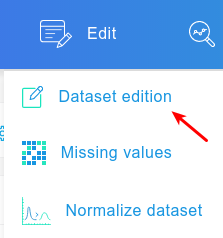
16.2 Edition
The module is reached this way:
We select the dataset, then pick the action rename categories, write names instead of numbers in the boxes, and click on Run, as shown below. Here, LumA stands for Luminal A and LumB for Luminal B.
We then save the new dataset.

And we rename it.
Here is the result in the workspace:
Now that we have the subtypes, let us start our exploration of mrna.
16.3 Principal Component Analysis (PCA)
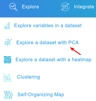
Since mrna has 2000 variables, we won’t explore bivariate relationships pair by pair. Rather, we will use PCA because it determines the best linear combinations of variables in terms of variability. We enter the PCA module this way:
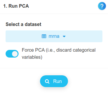
After selecting the mrna dataset, we click on Run:
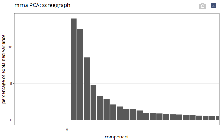
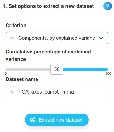
On the screegraph, we can see that the percentage of explained variance decreases rapidly with the component number. Were we to select a few components for exploration purpose only, we would pick 3 or 4 of them, based on the “elbow” rule. In this case, we will instead pick as many components as necessary to reach a cumulative explained variance of 50%. This way, we will not only be able to explore individuals based on the first few components, but we will also be able to perform a clustering analysis on a much reduced set of variables (i.e. on a few components).
Since we are only interested in getting the principal components, let us extract them by going to the appropriate menu:

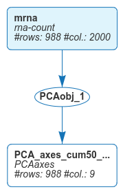
We then extract the dataset after selecting the criterium Components, by explained variance. The cursor used to select the cumulative explained variance is already on 50%. We eventually get the first 9 principal components.
Here is a selected view of the workspace, with the PCA analysis and the extracted dataset:
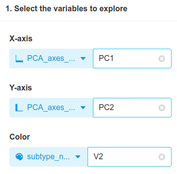
Now, we would like to plot individuals on these components, and link them to the subtypes. To get multivariate plots, let us go to the appropriate module in ASTERICS:
Then to the submenu with up to 5 variables:

This menu enables us to get a bivariate plot on which we can add colours, shapes and sizes. We’ll plot the first 2 principal components and add subtypes as colours.
Here is the result:
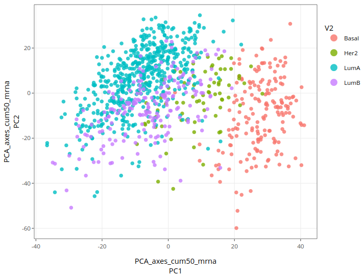
Basal subtypes are quite well separated from other types, whereas Luminal-A and B are difficult to distinguish from each other. Her-2 cases are not clearly distinguished from other types. This result makes sense biologically since Luminal types (A and B) are the most similar in terms of mechanisms, whereas Basal types are quite different (and are considered the most aggressive). Even though not perfect, a link between mRNA data and subtypes can be seen on the plot. The goal is now to improve this result, if possible. One way could be to use a clustering method since it directly outputs groups and not components.
16.4 Hierarchical clustering
We first enter the clustering module.
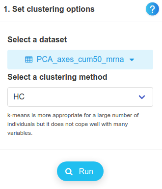
After selecting PCA_axes_cum50_mrna (as a reminder, it contains the first 9 principal components from mrna), we click on Run.
We then go to the next menu.

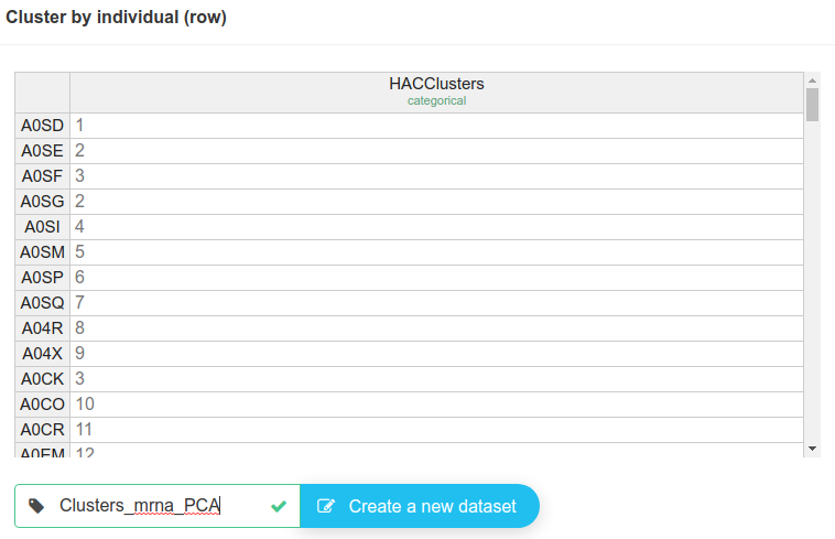
We choose to keep 36 clusters, based on the broken stick method. Once we have clicked on Explore, we go directly to the Clusters submenu.

And we extract them, after renaming the dataset for more clarity.
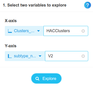
We want now a bivariate analysis, to compare clusters and subtypes. We go to the module to explore variables, and to the sub-menu with 2 variables:

We’ll look at the counts of individuals in each cluster, and colour them with respect to cancer subtypes.
Here is the result:
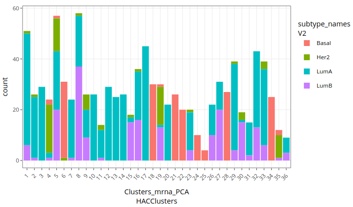
Several clusters (6, 18, 21, 22, 24, 25, 28, 34) seem to identify Basal subtypes well. A majority of Her-2 cases are mixed in different clusters. Luminal-A and Luminal-B are often mixed together and can’t be clearly distinguished, although a number of clusters approximately identify Luminal-A cases (1, 2, 3, 7, 10, 11, 12, 13, 14, 17, 20, 23, 29, 31, 33).
We leave the clustering analysis on the full mrna dataset to the interested readers. It should lead to similar observations.
This analysis shows again a link between subtypes and mRNA data, although its results are not clearly better than those of the PCA alone. Another possibility for improvement is to use miRNA data, which we haven’t loaded yet, and perform a multiple factor analysis. Let us load the data.
16.5 Data import
In the workspace, let us click on the Add button,
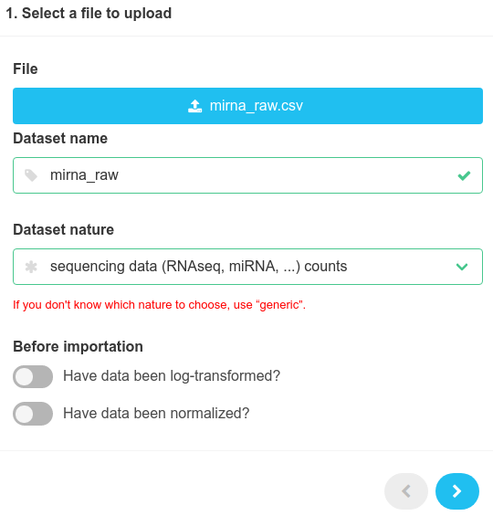
and load a file called mirna_raw.csv (that can be found at https://doi.org/10.15454/YNMQUY).
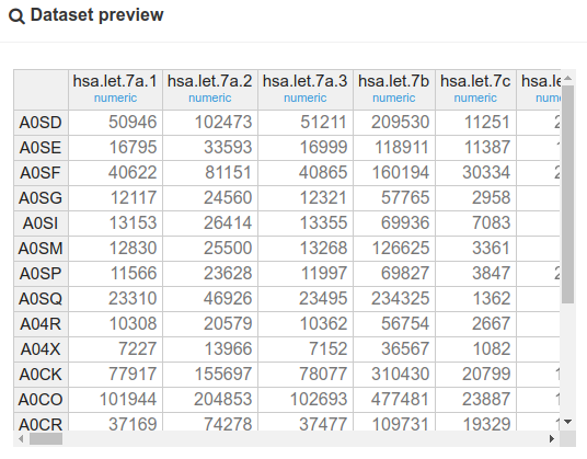
Below is the dataset preview.
Let us click on
 and see the result in the workspace.
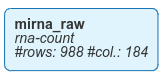
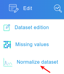
As can be seen in the preview above, the data comes in the form of raw counts, which we would like to normalize in approximately the same way as mrna (on which was applied a series of operations containing an upper quartile normalization, a division by the library sizes and a log-transformation). In this case, we will reproduce these operations on mirna, but instead of using an upper quartile normalization, we will compute TMM factors, which serve the same purpose of normalizing the library sizes and have been shown to have some advantages (Dillies et al. 2012). To this end, we will use the normalization module.
16.6 Normalization
From the workspace, the module is reached this way:
Selecting several datasets in turn should show that we are offered different normalization options, hence the importance of the data nature given to a dataset when importing it. We select RNAseq normalization (TMM), as shown below.
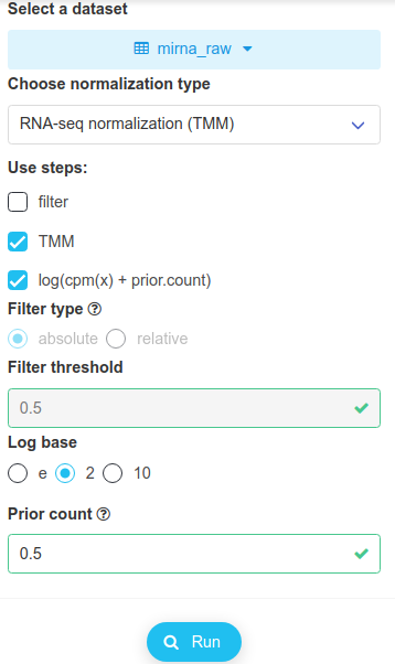
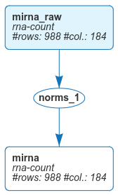
Note that filtering has been disabled in this case. After clicking on Run, we save the dataset and name it simply mirna.

Back to the workspace, we can see the new dataset.
16.7 Multiple Factor Analysis (MFA)
Let us now go to the MFA module.
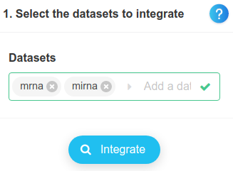
We integrate mrna and mirna.
We then go to the next menu.

And click on Run.

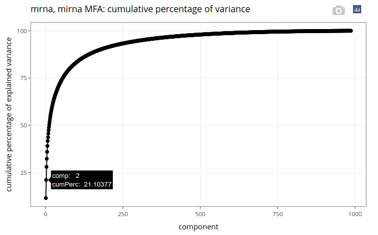
We get a cumulative variance plot, on which we can read that the first 2 principal components account for more than 21% of the total variance in the datasets.
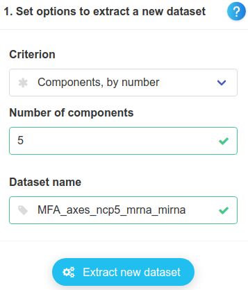
We then go to the extract menu.

There, we extract the components, without changing any parameter.
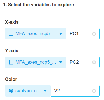
Back to the module to plot variables, we use the newly extracted components and the subtypes as colours.
Here is the result:
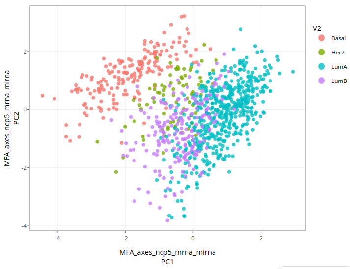
Basal types are still quite well separated, while Luminal-B cases are again mixed with Luminal-A and Her-2 cases. Visually, MFA using mirna does not seem to have improved the link between data and subtypes in comparison to what we have seen so far. Could we do better ? For the time being, we have only used unsupervised methods, i.e. that do not use subtypes. Let us then try a discriminant analysis.
16.8 Partial Least Squares - Discriminant Analysis (PLS-DA)
Let us now go to the PLS-DA module.
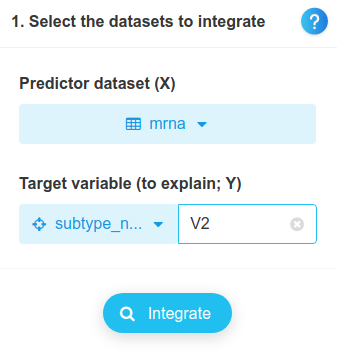
We integrate mrna and subtypes.
We then go to the next menu.

There, we click on Run.

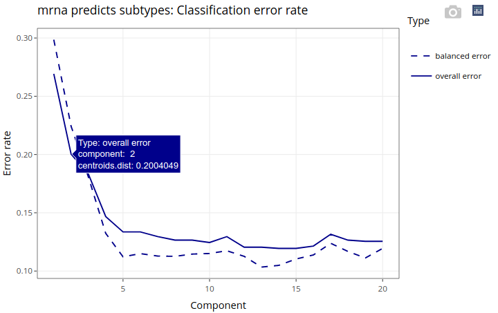
Note that the classification error rate is at about 12% using 10 components, and it is already as low as 20% only using the first 2 components, which we will look into.
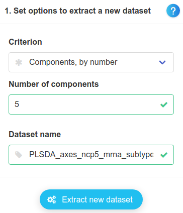
We then go to the extract menu.

There, we extract the components, without changing any parameter.
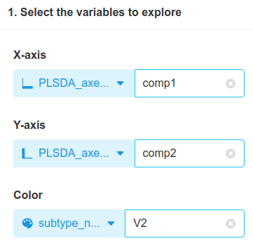
Back to the module to plot variables, we use the newly extracted components and the subtypes as colours.
Here is the result:
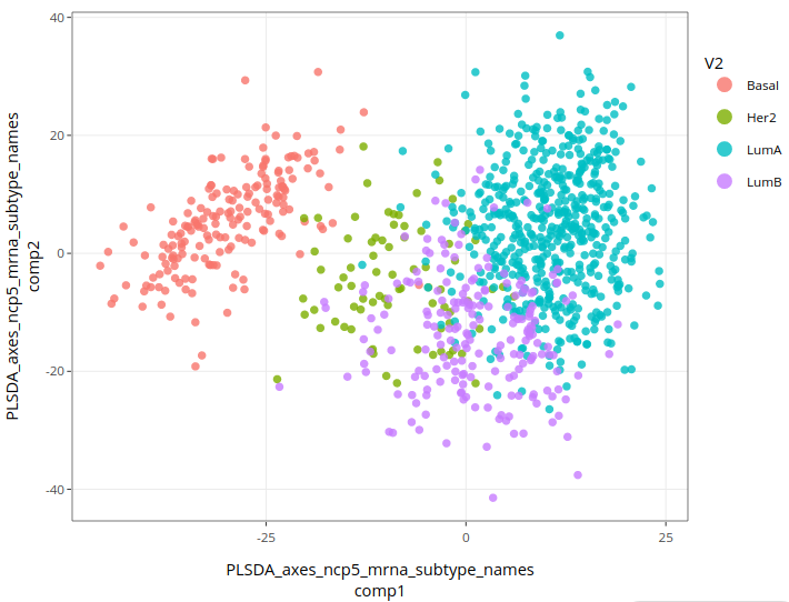
This is the best result so far, mostly because Luminal types are better separated from each other. Basal type remains well separated from other types, while Her-2 cases still lie in between. This good result is not a complete surprise since PLS-DA uses the subtypes to find components. Nevertheless, it is remarkable to find a plane in a 2000 dimensional space that offers such a good separation between cancer subtypes.
To make sense of this result, we would have to investigate both components, trying to identify genes whose expression levels are correlated with cancer subtypes. Let us start this exploration here.
16.9 Interpretation
We go back to the PLS-DA module and to the menu Explore variables.

There, we click on Plot variables, without changing the settings. A correlation circle is drawn, with variables (genes) whose correlations with the first 2 components are above a threshold (0.8 by default).
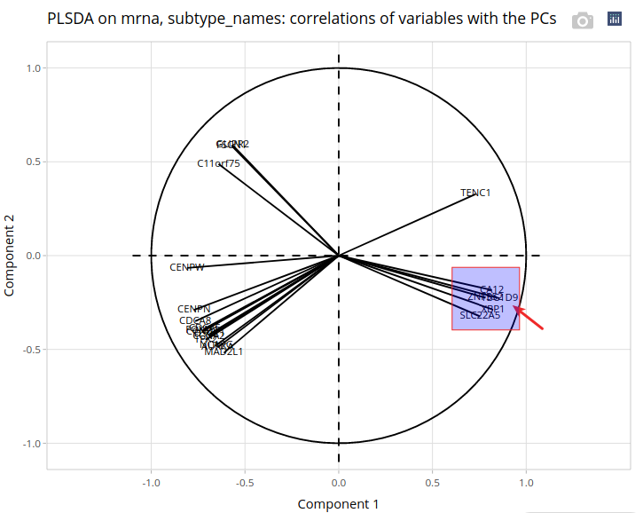
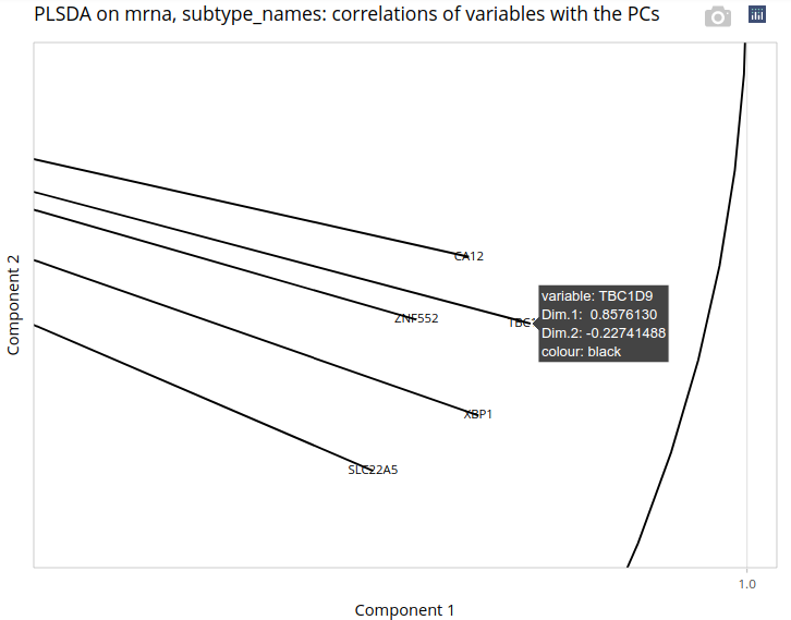
Since variables with a large correlation with one component are the most helpful to interpret it, we will focus on TBC1D9 - the gene shown by the arrow, whose correlation with the first component reaches 0.86. Explaining the first component is particularly interesting in our case since it distinguishes Basal cases from other cases. Indeed, the plot of the individuals on the first 2 components shows a separation between cases that is mostly determined by the first axis. Let us zoom in on the correlation circle.
Now, let us go to the module to plot variables, and to the menu for 2 variables. We will plot the normalized expression of TBC1D9, split by subtype.
Here is the result:
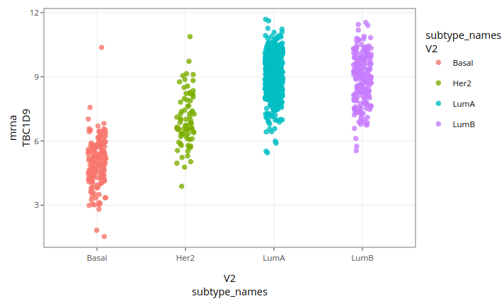
Basal cases correspond to low gene expressions and Luminal cases to high expressions, while Her-2 cases lie in between. This is consistent with the plot of individuals on the PLS-DA components. The first component is thus partly explained by the expression level of TBC1D9, but it is not limited to it. On a final note, let us mention that our analysis limited itself to finding a set of discriminant genes and that it could be completed by statistical tests on individual genes to verify that their levels of expression between subtypes are significant. It happens that the gene we just studied have been identified as differentially expressed between breast cancer subtypes in a previous article (Kothari et al. 2021).
16.9.1 Conclusion
We wanted to explore the relationship between breast cancer subtypes and omics data. After our analysis, we can say that the relationship between subtypes and mRNA (and miRNA) is rather strong. Moreover, this relationship can be well described linearly since PLS-DA yields a test error rate of about 12%. Finally, although our investigation remained very limited, it seems that our results are consistent with other works on cancer subtypes and related gene expressions.