Section 14 Partial Least Squares - Discriminant Analysis (PLS-DA)
Performs Partial Least Squares - Discriminant Analysis on two datasets.
Integrate two datasets with PLS-DA, a supervised approach to project individuals described by numeric variables (in a first dataset, X) on a subspace where they are separated at best based on their value for a categorical variable (in a second dataset, Y).
- Pre-processing to ensure individuals of both datasets match (numerical description of combined datasets, Venn diagramm and upset plot)
- (Similarly to PCA) Graphical outputs: screeplot, projection of individuals, projection of variables on circle of correlation.
- Possibility to extract a new dataset based on PLS loadings or on selected variables.
The method used in ASTERICS comes from the mixOmics (Rohart et al. 2017) package.
For further information on PLS-DA method:
14.1 Preprocessing

PLS-DA uses two datasets: X contains numeric variables in columns (e.g.,
gene expression), and Y contains one column (other columns can be present but
will not be used) that is a categorical variable (e.g., treatments or other
information on the design of the experiment) that is to be discriminated at best
using the variables in X. In short, each row of Y describes to which group the
corresponding individual belongs and X is used to discriminate these groups.
Since X and Y are in two different datasets (dataset1 and dataset2 below),
only individuals common to X and Y are used in this analysis.

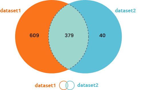
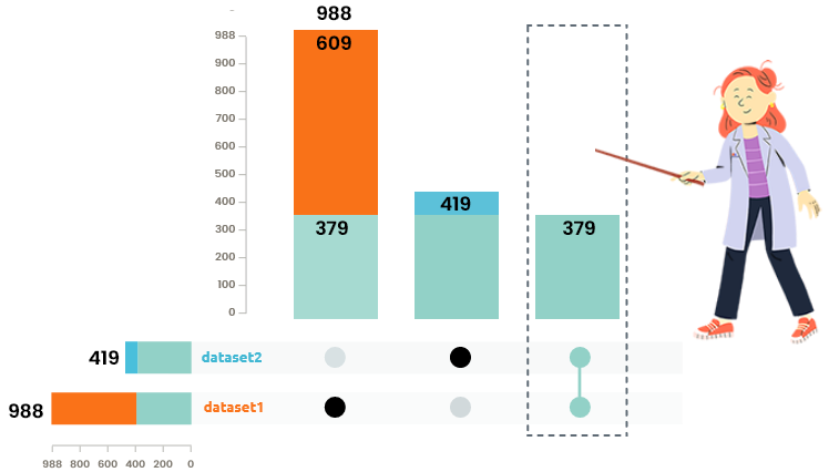
Venn diagram and upset plots are used to understand how many individuals are common / specific to each dataset. Only individuals common to all integrated datasets are used in the analysis.
14.2 Run PLS-DA
How to set options? Now that your datasets are ready to be used, click on the left panel to start PLS-DA and wait for the computation (that can be a bit long).
Important note: PLS-DA is performed with raw values (data are not scaled to unit variance before they are processed). If you want to perform PLS-DA on scaled data (predictors only), go to the menu “Edit / Dataset edition” and scale your dataset before PLS-DA.

Quality of the PLS-DA is given by the classification error rate. A classification error rate equal to 0.15 means that predicting the target variable with PLS-DA leads to 15% of wrong predictions (based on 5-fold cross-validation strategy). The “Classification error rate” plot is used to choose the number of components in PLS-DA as the one minimizing the error rate. The balanced error rate is a complementary information where error rate is the average of the error rates for all the levels of the target variable. It is especially useful when the target variable has very unbalanced number of observed individuals between levels.
Contrary to PCA, reproduced inertia is not an objective of PLS-DA that finds the projection best suited to distinguish between levels of the target variable. These plots are given as mere information but can not be directly use to choose the number of PLS components.
14.3 Explore individuals

Similarly to PCA, the interpretation of PLS-DA is done component (axis) by component, starting from the first which displays the main trends, in the numerical dataset, separating the individuals with respect to their levels for the target variable.
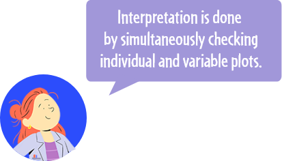
Combine the plot of individuals with colors (or shapes / sizes) giving information on other variables (e.g., variables of your design) to check if colors are organized with respect to components. This would mean that the main relationships between the variables from your two input datasets are also associated with the variable that has been used to color individuals in your plot.
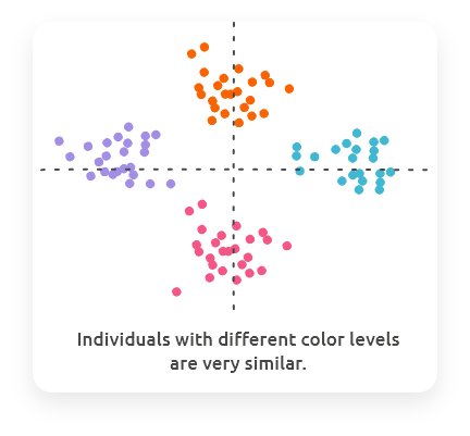
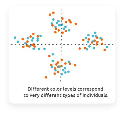
By default, the individuals are colored by their levels for the target variable and can help identify if PLS-DA results are relevant or not:
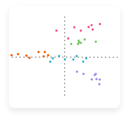
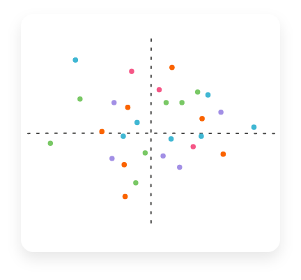
Individuals with different levels for the target variable are well separated on the individual plot: PLS-DA is probably a good prediction model.
Individuals with different levels for the target variable are not well separated on the individual plot: PLS-DA might not be relevant for these data (and its predictive power is low).
14.4 Explore variables
How to set options?
By choosing a correlation threshold, only variables with a correlation larger than this number are displayed on the plot (to make it easier to read).
Only variables well correlated with axes can be interpreted. Select a correlation threshold to display the most correlated variables.
14.5 Extract new data
How to set options?
Set options in left panel to generate a new dataset from the analysis:
with the criterion “Components, by number,” the first components (number to be specified by the user) will be extracted and used as a new dataset;
with the criterion “Components, by explained variance” (when available), the first components (number automatically set to reach the targeted percentage of explained variance or a targeted correlation ratio for categorical variables) will be extracted and used as a new dataset;
with the criterion “Variables,” the variables the most correlated with the first components will be selected and used as a new dataset.
When the dataset is extracted, you can use it in other analyses or check it in menu “My workspace.”