Section 17 Case study: Piglet
This case study focuses on fetal development in late gestation in pig species (Lefort et al. 2020). The study addresses the question of delayed development in mammalian that may impact survival ability at birth. Two ages at late gestation were studied, 90 and 110 days (birth is expected at 114 days). Two genetic lines were included, LW for Large White, with higher risk of delayed development, and MS for Meishan, more robust. Studied piglets were of four genotypes: LWLW, MSMS, and the crossed piglets LWMS and MSLW.
The data are gathered in nine datasets. Metabolomic analyses (NMR) were performed on plasma, urine, and amniotic fluid samples of 444 piglets. Transcriptomic and proteomic analyses were performed on a subset of 50 samples of muscle, liver, and blood. Two other datasets contain information on piglets, one limited to the subset of 50 piglets and the other for the 444 piglets. These two datasets do not contain the exact same information.
The case study is organized around biological questions ASTERICS contributed to answer.
17.1 Import data in ASTERICS
From the Workspace screen, click on Add to import a dataset:

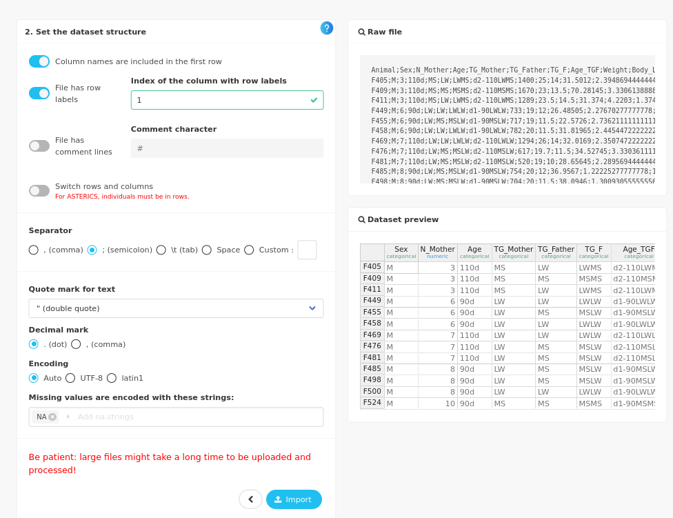
and provide the characteristics of your input file (semicolon as separator for instance). The dataset is ready to import when the Dataset preview on the left hand part of the screen is consistent with your data. Click on the Import button.
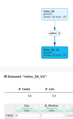
The dataset now appears in the workflow.

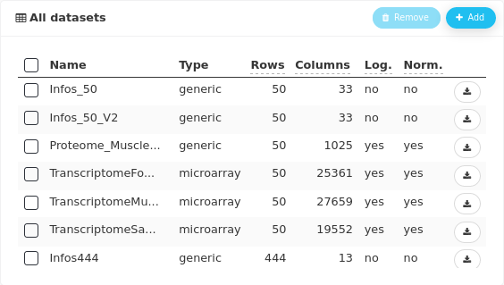
and in All datasets.

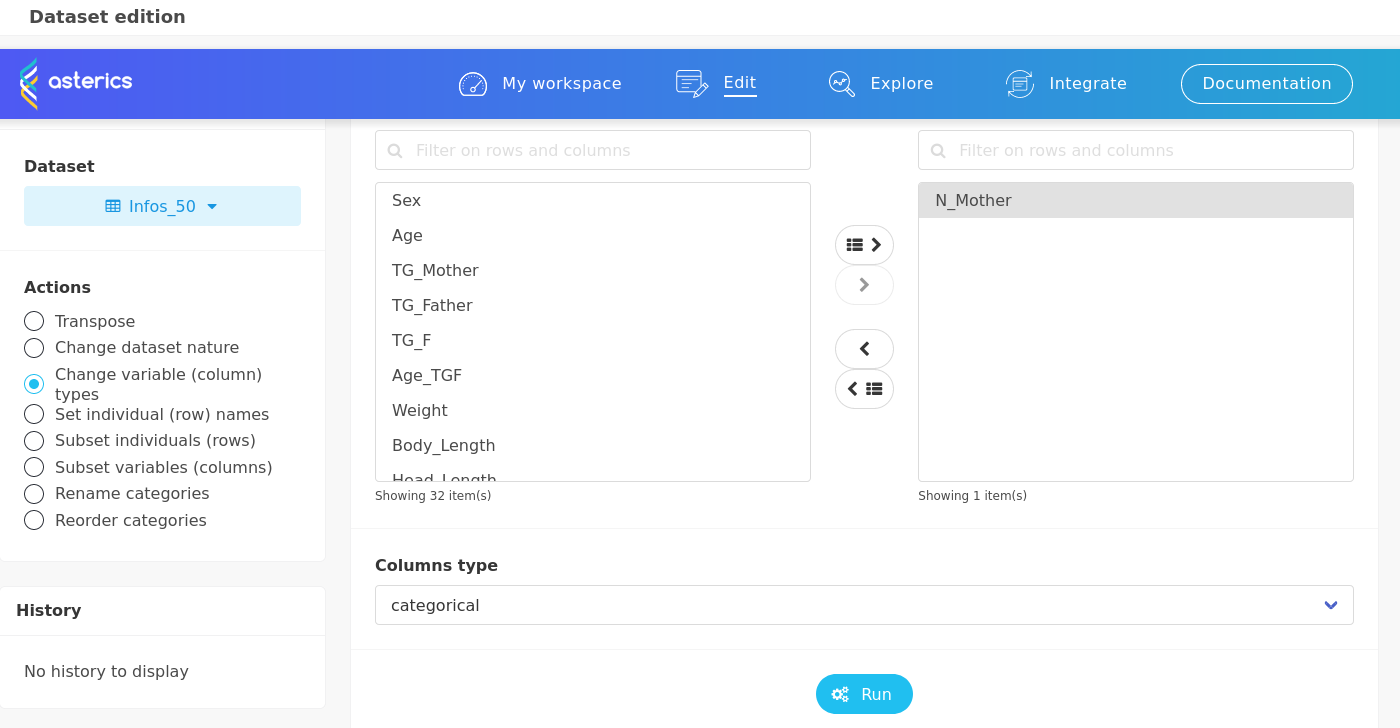
In the Dataset preview, it can be seen that N_Mother is considered as numeric. But, as it is an identifier, it has to be considered as categorical. This can be changed in the Edit menu.
The interface is rather intuitive to achieve such a conversion:
Do not forget to save the new dataset (otherwise, it will not be usable elsewhere)

under a new name
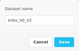
The new dataset now appears on the workflow linked to the original dataset through an editor analysis and N_Mother is now well considered as categorical in the new dataset called Infos_50_V2.
In the present study, several datasets were generated for the same 50 animals. They can be imported following the same process as described above.
As it is mentioned in the panel Set the dataset structure, For ASTERICS, individuals must be in rows.

Among the datasets that we want to import, some contain individuals in columns, and we thus have to switch rows and columns for them (as shown above).
When importing the datasets, details about normalization and log-transformation must be given. In our case, proteomics and transcriptomics datasets were log-converted and normalized before importation; metabolomics data were normalized.
The information about log-transformation and normalization of thdatasets can be checked after importation in the All datasets panel.
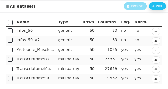
Note that the five imported datasets and the edited one all have 50 rows corresponding to the number of animals. In ASTERICS, correspondance between datasets is done by row names (if provided) or the rows are supposed to be ordered identically (if none has row names).
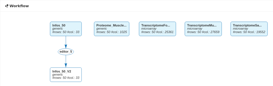
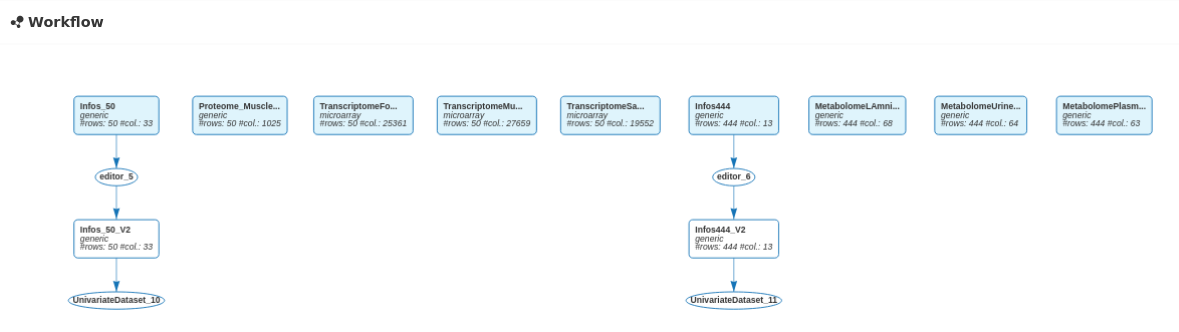
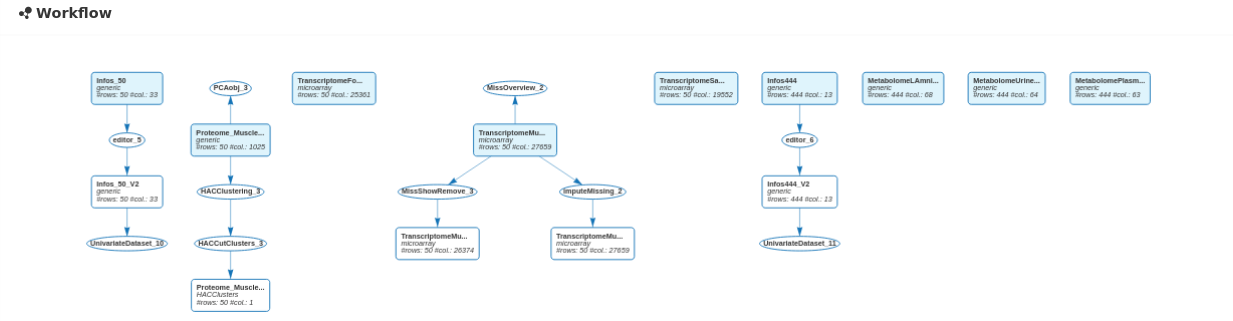
The six datasets are also visible in the workflow.
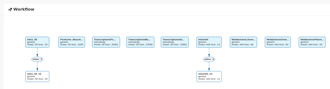
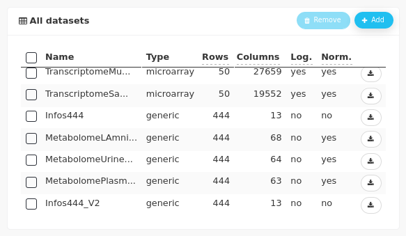
After importing the data for the 444 animals and editing the Infos_444 dataset to convert N_Mother in categorical, 11 data sets are visible in the workflow:
and in the All datasets panel:
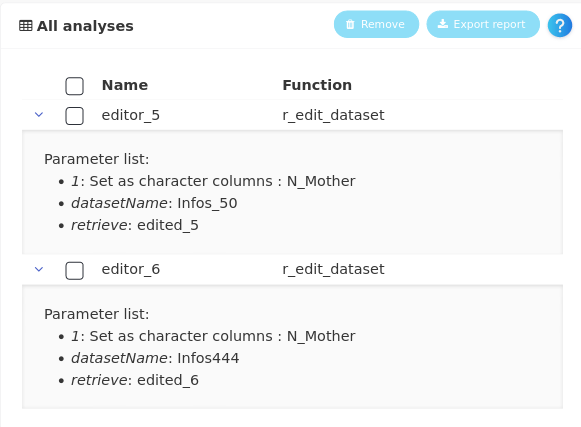
Furthermore, the two editions (changing the variable type for N_Mother) that we have performed appear in the All analyses panel, with the details of the analyses.
17.2 Univariate analyses
A univariate analysis is useful to have a quick look at one specific variable. It can be done as a prior analysis with our favorite variable(s). It can also be done after other analyses to investigate more precisely on a specific feature.
Univariate analyses are available in Explore variables in a dataset in the main menu Explore.
Let us illustrate this analysis with the variable Weight of the dataset Infos_50. It is a numeric variable, corresponding to the main trait available for all newborns in mammalian species and relevant to assess piglet survival.
17.2.1 Infos_50 Weight
Obtaining the univariate analysis of one variable is intuitive using the interface:

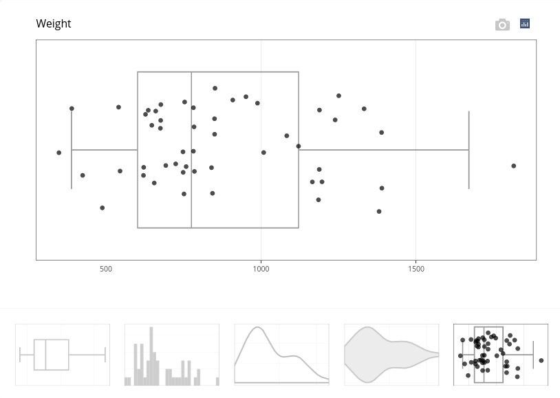
Obtained results contain plots:
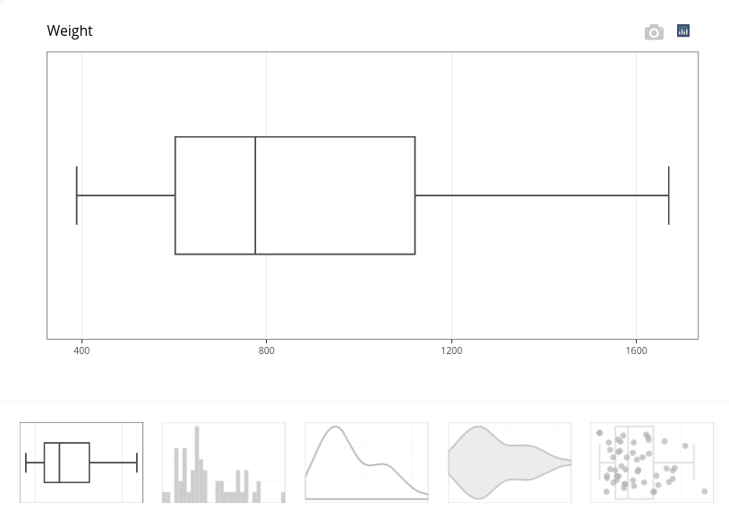
This boxplot illustrates the variation of weight. Other graphical outputs are available. For instance, the fifth plot in the bottom menu adds points to the boxplot.
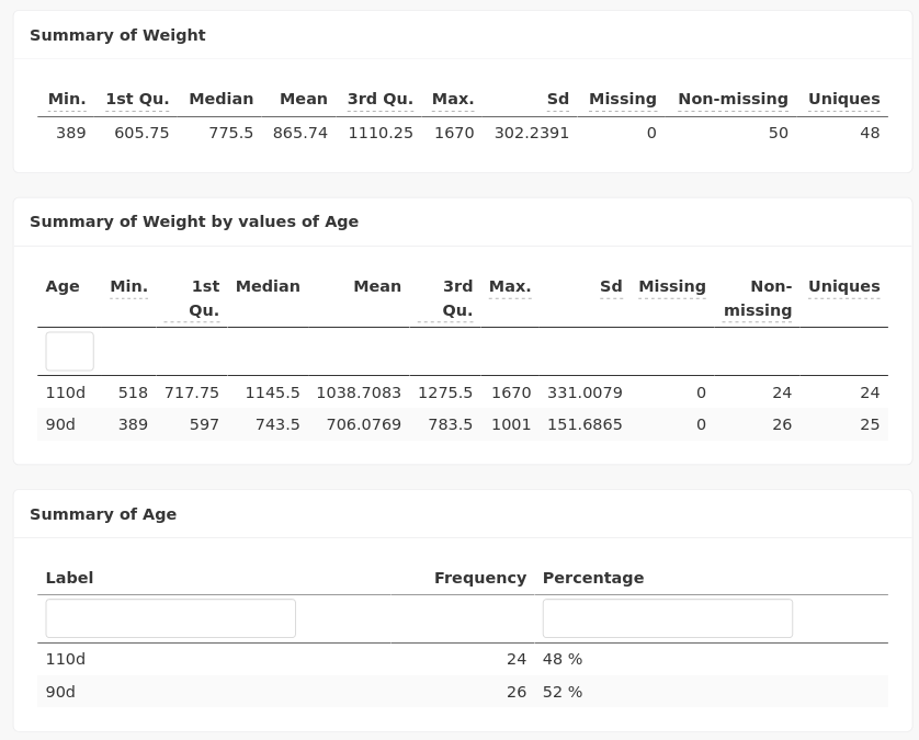
A numerical summary is also provided, which states that weights vary between 389 and 1670 with a mean of 865.74 (in gram):
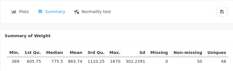
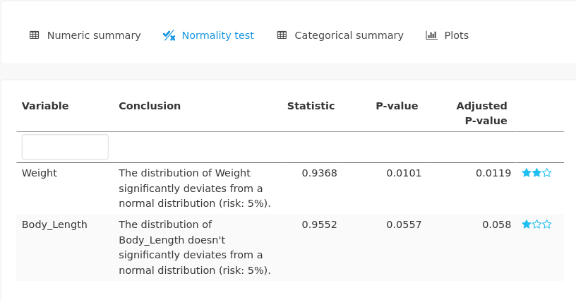
As it could have been suspected with the graphical outputs, the \(p\)-value of the normality test indicates that the distribution of Weight significantly deviates from a normal distribution:

Anymay, knowing that there are two ages of gestation, it is expected that this variable can have a bimodal distribution.
17.2.2 Weight and Age
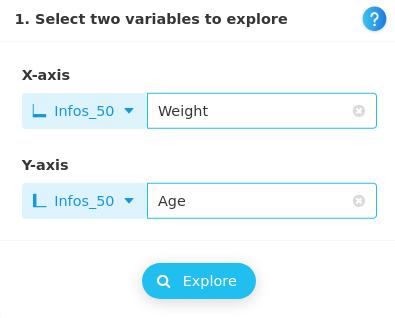
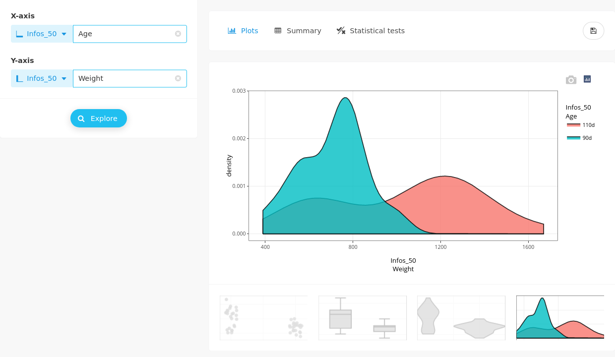
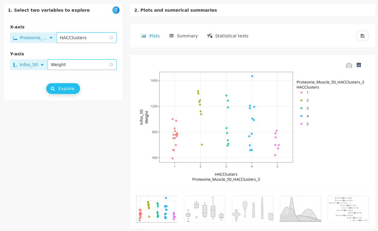
So we now investigate both variables Weight and Age simultaneously. It can be done in the Explore variables in a dataset, in the panel 2 variables:
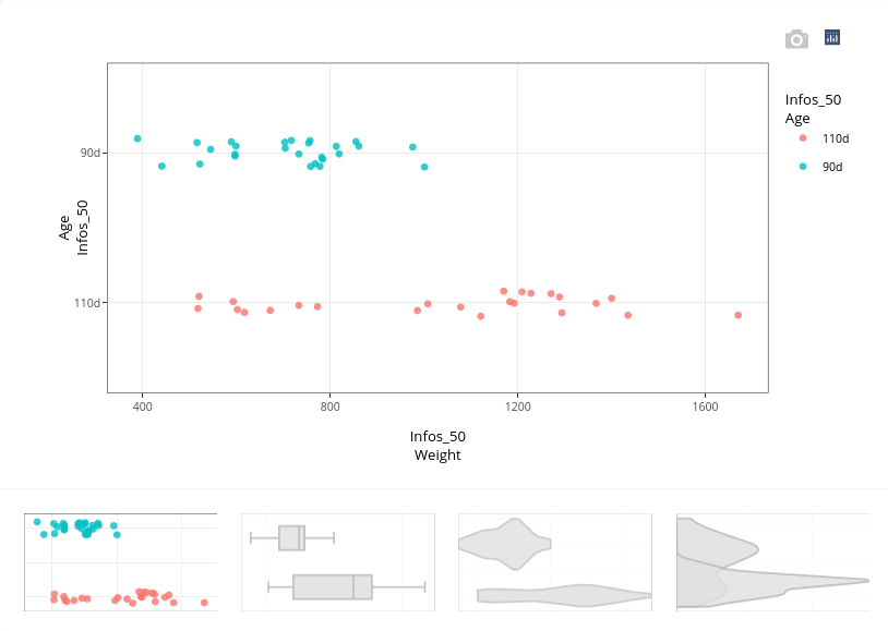
The plot illustrates the variation of weight in relation to the age of piglets (and it is interactive: when you position the cursor on one of the point, you can identify to which individual it corresponds). Obviously, at day 110, piglets weight more than at day 90. In contrast, some piglets at day 110 have the same weight that piglets at day 90. On the whole, the heterogeneity of weights is higher at day 110 than at day 90. Age 110 is the end of gestation (birth is expected at day 114). Hence, piglets not gaining weight at the end of gestation may have stunted growth, which may affect their ability to survive at birth.
Other graphical outputs (boxplots, violin and density plots) can complete the overview. For the density plot, it can be more natural to switch X and Y axis to display the density in a more conventional way.
Numerical summaries are also available:
as well as various statistical testing, here for normality, and the effect of the categorical variable (Age) on the numerical one (Weight), with parametric (ANOVA) and non parametric (Kruskal-Wallis) tests. Here, KS test results should be prefered since the normality assumption is rejected.
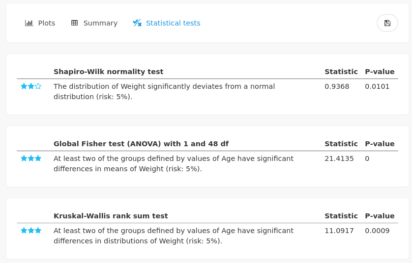
As it could be expected from the graphical outputs, the distribution of the weight between the two groups of ages are significantly different.
17.2.3 All variables in Info50
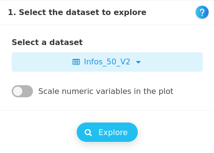
A univariate analysis of every variable of a dataset can be performed at once using All variables in a dataset. We just have to provide the dataset, here Infos50_V2 including the conversion of N_Mother to a categorical variable.
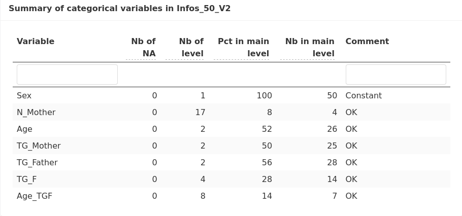
Some specific variables are automatically excluded from the analyses, for instance when a categorical variable has a unique value, as in our case with the variable Sex (all the 50 individuals are males):

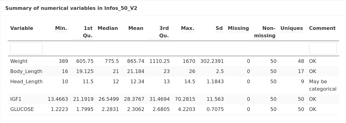
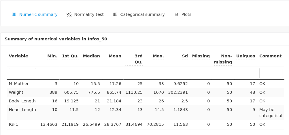
A summary of numerical variables is provided:
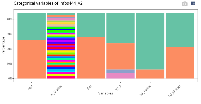
as well as a summary of categorical variables (including N_mother):
Normality tests are also provided for every numerical variable:
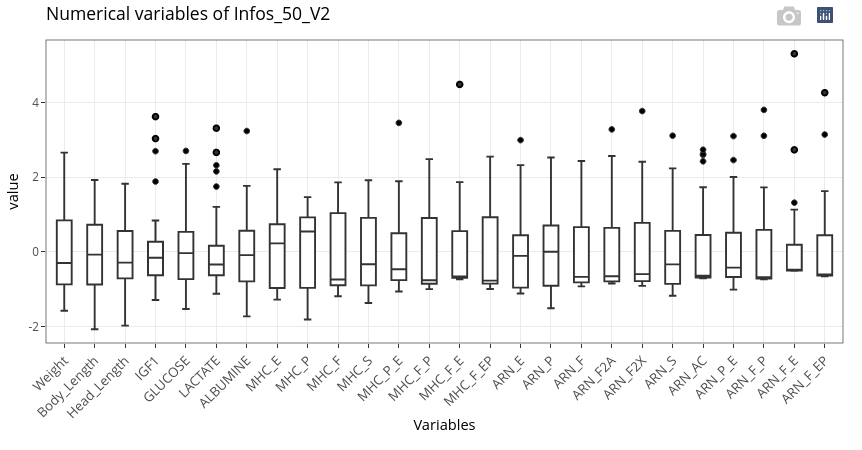
Parallel boxplots are displayed for the numerical variables:
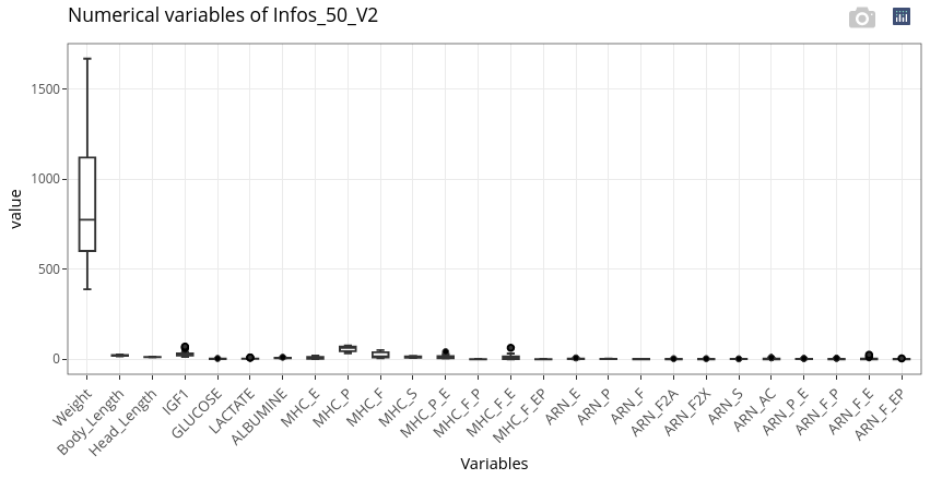
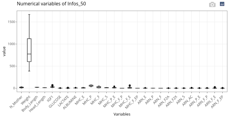
If numerical variables have too different orders of magnitude (as here with Weight compared to the other features), it can be relevant to scale the data to get a more meaningful graphical output.

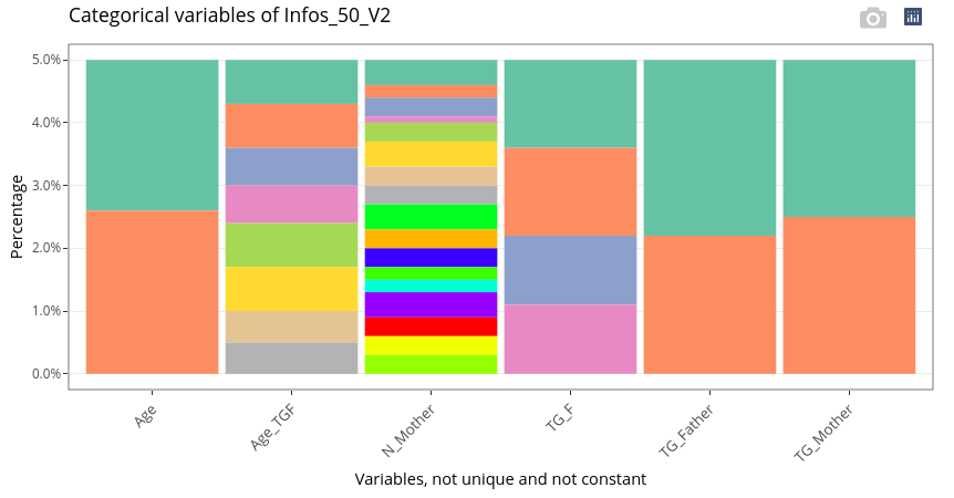
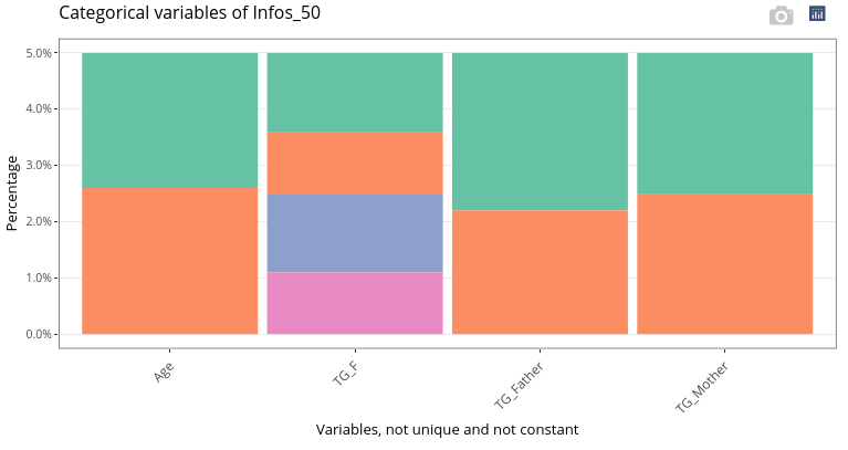
Categorical variables (including N_Mother) are displayed as stacked barplots.
If we hadn’t changed the type of N_Mother, or if we run the analyses with Infos_50, means and standard deviation of N_Mother would have been computed (which would have had no meaning):
and the variable would have been included in the boxplots:
and not with categorical variables:
17.2.4 Correlation plot of a dataset
An image of the correlation matrix can be displayed in the panel Correlation plot of a dataset.

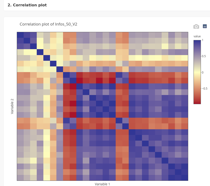
The correlation matrix is interactive and the names of two variables corresponding to a correlation value are visible when the cursor is positioned on a square of the matrix.
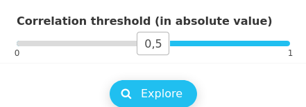
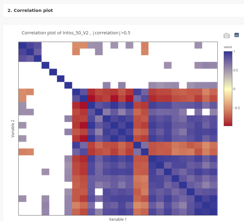
A slider enables to set a threshold to display only correlations higher than this specific value. The cells corresponding to correlations lower than the threshold are displayed in white.
17.3 Missing values (NA for Not Available)
If a dataset contains missing values, it can be useful to deal with them specifically, as most statistical methods in ASTERICS require complete datasets to be run.
To do so, a dedicated module is available in the Edit panel.

Let us illustrate it with the Transcriptome_Muscle_50 dataset.
17.3.1 Explore NA
First, the distribution of missing values in the dataset can be visualized. When the number of variables is large (as for the Transcriptome_Muscle_50 dataset with more than 20,000 variables), the graphical output has to be adapted.

Two heatmaps are provided to give a global overview of missingness pattern in the dataset. The first one keeps the rows and the columns in the same order as the analyzed data table.
![]()
The second one is reordered according to the percentage of missing values.
![]()
Other plots can be checked to reveal missingness patterns either by variable
![]()
or by individual
![]()
Once explored, a decision has to be taken: either remove variables or individuals with NA, or impute the missing values. Both strategies will provide a complete dataset.
17.3.2 Remove NA
Removing NA in a dataset can be done either in a strict way (moving the slider to 0% of acceptable missingness in individuals or variables) or in a softer way to keep some variables or individuals (change the direction) with few missing values. In this case, the resulting dataset can still have missing values after the filtering. Both options are available in the Remove missing values panel.
![]()
The strict way can be irrelevant as it can remove a huge part of the data. In our example, choosing the direction individuals would remove 43 individuals among 50.
![]()
It is more relevant to opt for the direction variables to remove “only” 1285 variables among more than 26000.
![]()
The removed and kept variables are displayed in a static heatmap of the dataset (which can sometimes be difficult to read when the dataset is large, as in our case).
![]()
To be used in further analyses, the complete dataset has to be extracted.
![]()
![]()
17.3.3 Impute NA
Three methods are available to impute missing values in the ad hoc panel. Have a look at the documentation to decide which method is adapted to your data. As an example, the summary of the imputation with PCA gives the following output:
![]()
As indicated, the dataset has to be extracted to be used for further analyses.
![]()
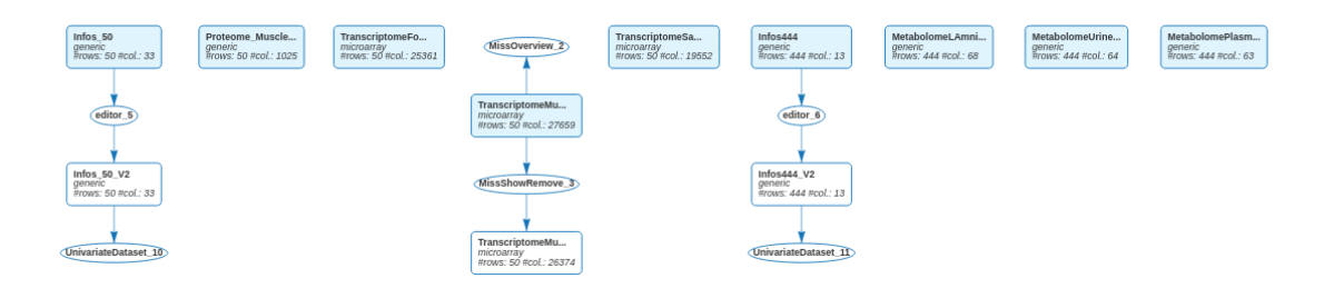
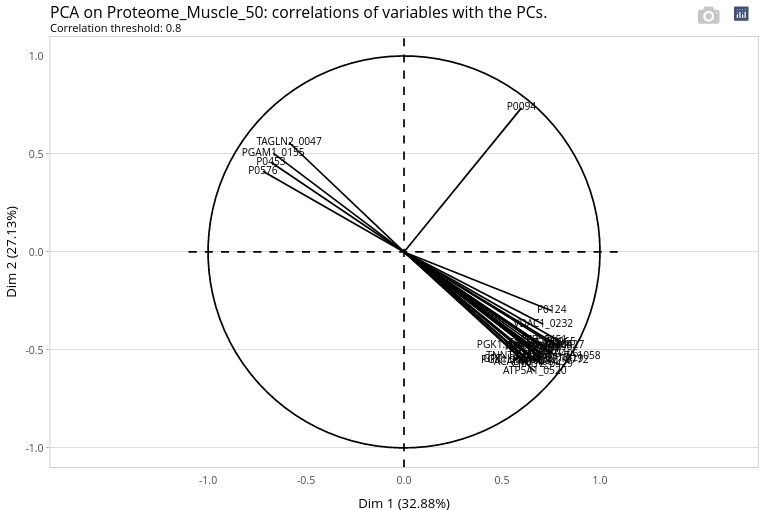
17.3.3.1 Workflow
The updated workflow clearly indicates that we have adopted two strategies to deal with the missing values of the Transcriptome_Muscle_50 dataset.
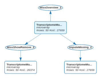
The two strategies could also have been used sequentially. First, remove rows and columns allowing a small percentage of missing values. Then, impute the remaining missing values to obtain a complete dataset.
17.4 Multivariate analysis with Principal Component Analysis
Principal Component Analysis (PCA) is in the panel Explore. Let us illustrate this method on the Proteome_Muscle dataset.
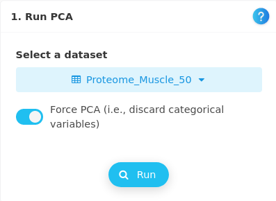
17.4.1 How many components?
When performing PCA, the first decision to take is the number of components to keep for graphical outputs. This choice can be oriented by taking a look at the screegraph.
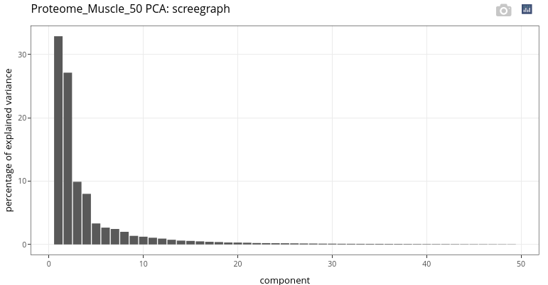
The large gap between the second and the third components leads us to consider two principal components for graphical outputs.
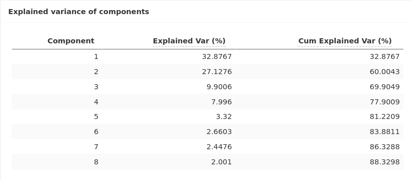
The inertia table indicates that we keep around 60% of the information with these two components.
Then, other graphical outputs, useful for the interpretation, are available in the ad hoc panels Explore individual and Explore variables.
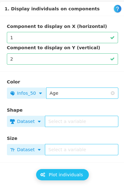
17.4.2 Individual plot
Here, the individual plot without any enhancement is not meaningful, except that we cannot identify specific shapes or patterns or outliers in the location of the points representing the individuals.
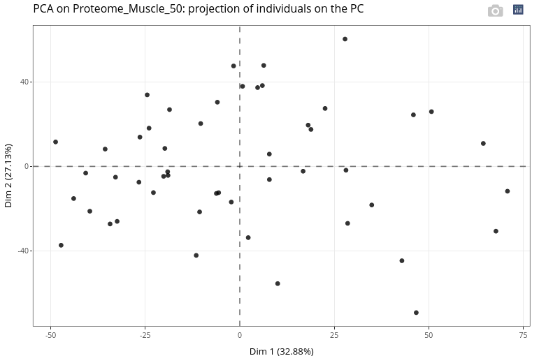
It is highly recommended to use categorical variables to modify color, shape and size of the points.
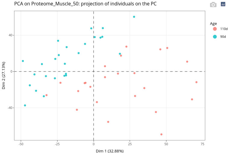
As expected, Age appears to have a strong effect on the variability in the data.
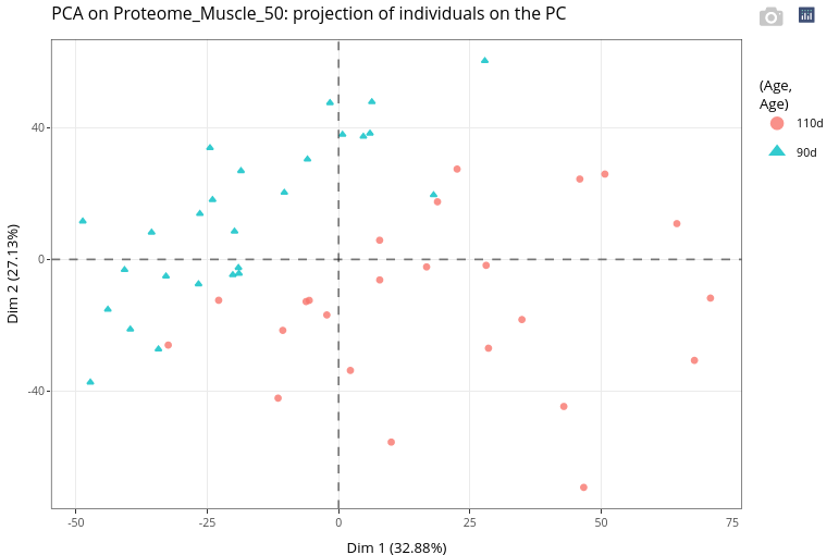
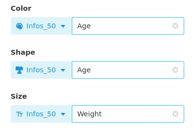
The same variable can be used for 2 different graphical features.

A numerical variable can also be used to set a graphical feature. We use the variable Weight to change the size of the points.
This could result in a graphical output relatively difficult to interpret.
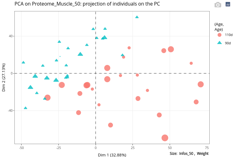
As expected, weights at age 110 are higher than at age 90. Nevertheless, the weight does not seem to explain the heterogeneity at age 110, i.e., higher weights are not positioned at an extreme (left or right) of the first axis, nor at an extreme of the second axis.
17.4.3 Variable plot
Use the slider to lower the number of displayed variables. The higher the correlation, the lower the number of displayed variables.
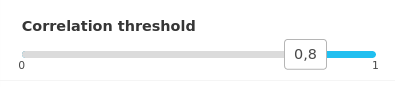
We can observe that some proteins are very correlated to the first axis with a correlation higher than 0.9. These proteins may be quantitatively very different at day 90 and et day 110. This could be confirmed with the statistical analysis in the menu ‘Integrate/Differential analysis’ (not shown).
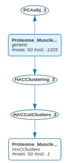
17.5 Clustering
We carry on the exploration of the Proteome_Muscle dataset addressing a clustering purpose: we want to cluster the 50 animals. Clustering methods are available in the Explore main menu.
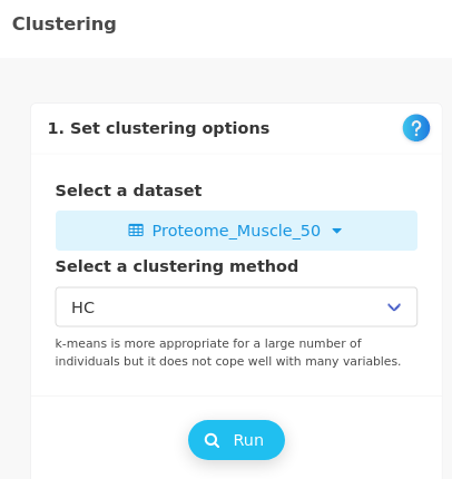
The first step consists in choosing the number of clusters in the panel Choose the number of clusters.
Biologically, we expect a number of clusters relative to the number of conditions. Here, we have two ages and we have four genotypes for the piglets. Then a number of clusters of 8 would be perfect but surprises are to be expected in biology.
Some heuristics to choose the number of clusters are also proposed in ASTERICS, such as the “broken stick” heuristic.
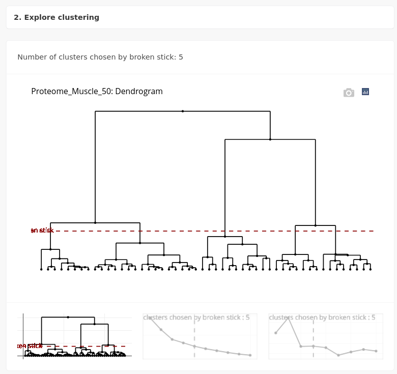
Here, five clusters are proposed, and we’ll explore them in the following with Make and explore clusters.
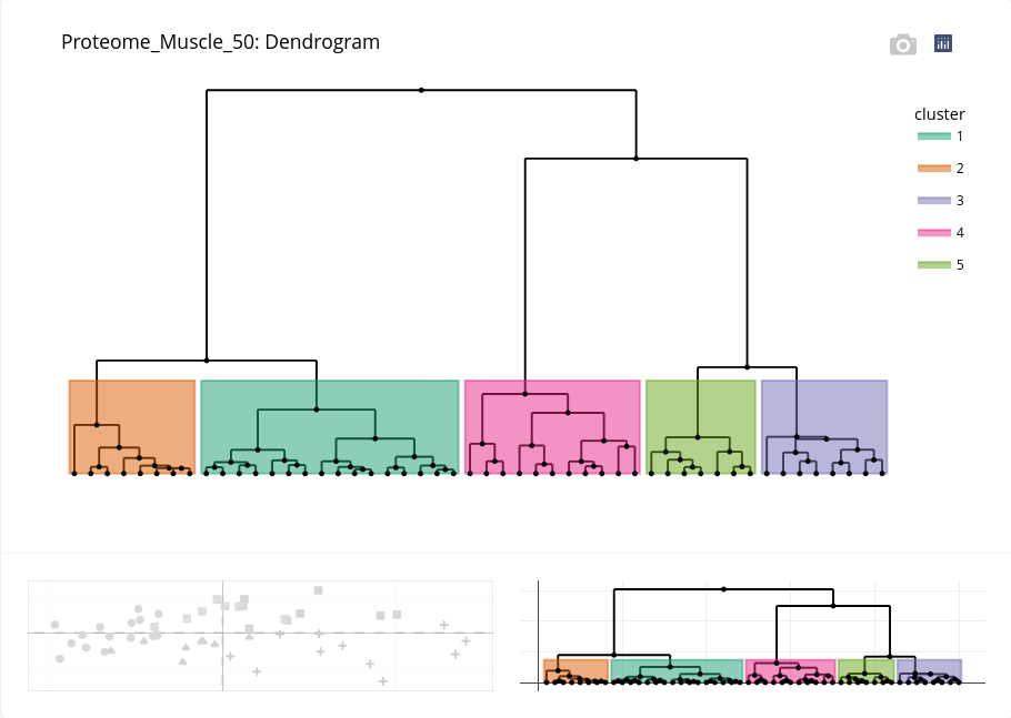
First, an enhanced dendrogram can be displayed to better highlight the clusters:
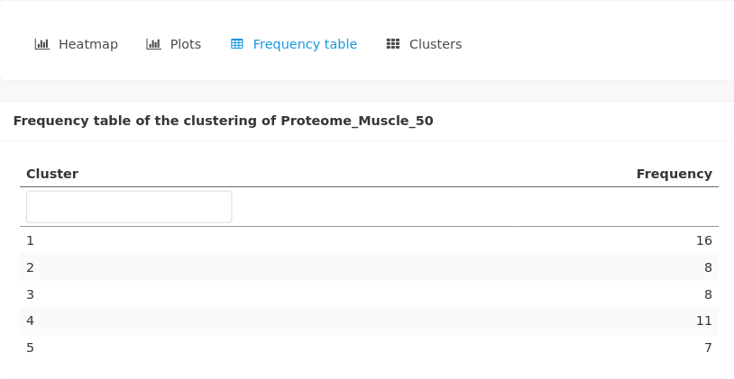
A table gives the number of individuals by cluster:
A plot of the projection of individuals on the first axis of the PCA is also given, with the colors of the points corresponding to the clusters.
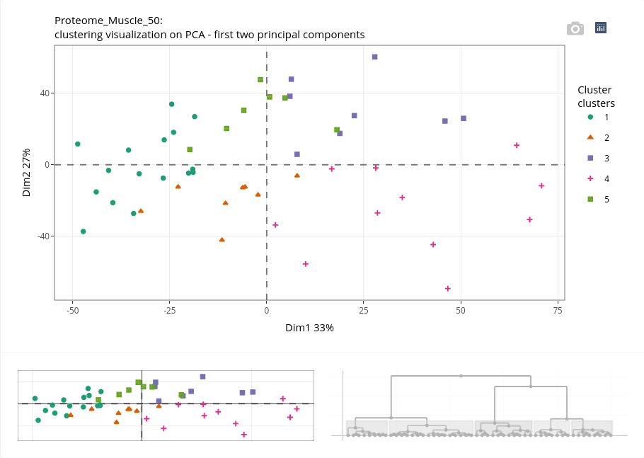
If we have kept in mind the former PCA projection of individuals, we can deduce that the cluster 1 is composed of piglets at day 90, cluster 2 piglets at day 110, cluster 4 piglets at day 110, cluster 5 piglets at day 90. The cluster 3 is surprisingly composed of piglets at both ages! Further exploration may help to elucidate this clustering.
We can explore these clusters in the Explore variables in a dataset panel to test some variables already known to be important for piglet maturity. We will test genotype, weight, and also glucose, albumine, MHC_E (the embryonic myosin). To do so, we have to retrieve the cluster information to know which individual is in which cluster.
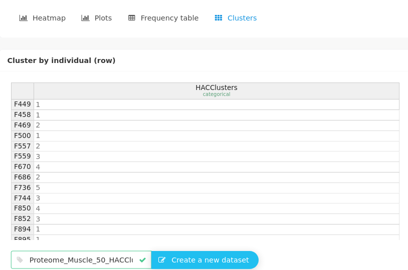
This information can be extracted to a new dataset and used in further analyses. For instance, explore 2 variables, one being categorical and indicating the cluster.
First, we cross the categorical variable Age with the clusters:
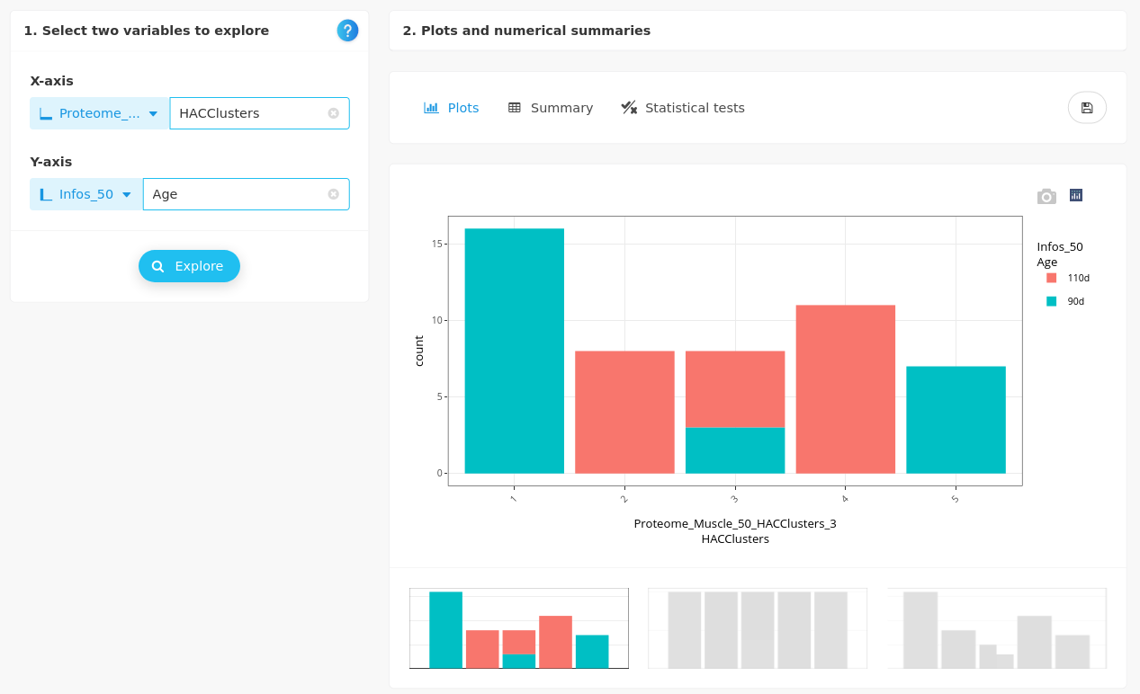
and then, we check their impact on two numerical variables from Infos_50:
- MHC_E
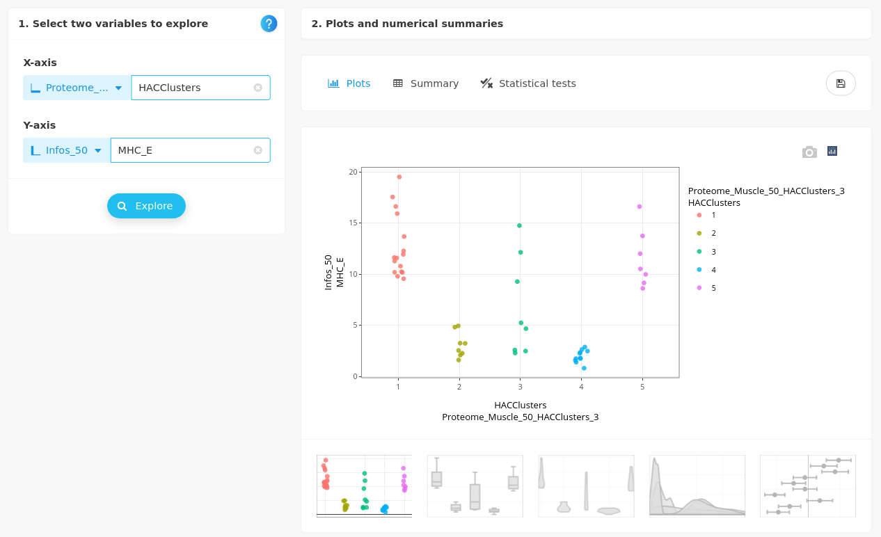
The embryonic myosin is more expressed at day 90 than at day 110. This variable is not helpful to explain cluster 3 but discriminates clusters 1 and 5 (90d) from clusters 2 and 4 (110d).
- Weight
The body weight does not explained the clustering either. Further investigations are needed to explain this clustering of piglets, that is probably the result of a complex combination of several characteristics.
17.6 Integrate two datasets with PLS
17.6.1 Proteome and Transcriptome Muscle 50 animals
We propose to explore the relationships between the transcriptome and the proteome of muscle tissus from the same individuals. To do so, we use one complete transcriptome dataset previously obtained by removing the columns with missing values.
17.6.1.1 Preprocessing
![]()
We first verify that we have exactly the same piglets studied and for how many variables. The two tables provided here are the same because the two datasets we want to integrate were acquired from the very same individuals (the matching criterion is the row names, as given during the importation of datasets: be careful to set this value properly before you integrate datasets).
![]()
This is confirmed with the Venn diagram.
![]()
17.6.1.2 Explore individuals
![]()
The individual plot clearly highlights two clusters. To elucidate this phenomenon, we can custom the individual plot to display some features.
![]()
As expected considering the previous analysis, the investigation leads to an Age effect.
Compared to the PCA, the differentiation between ages is stronger when combining the two datasets.
17.6.1.3 Explore variables
The variable plot can be difficult to interpret depending on the number of variables. It is recommended to use correlation threshold to lower the number of displayed variables.
![]()
Even with a threshold of 0.9, the number of variables remains very high for the transcriptome dataset. At this step, it is still difficult to infer biological knowledge. Further investigations are required to identify the most relevant transcripts.
17.6.2 Proteome Muscle 50 animals and Metabolome Plasma 444 animals
Now, we explore a tissue omic, proteome of the muscle, with a fluid omic, the metabolome of the plasma. This is could be interesting to investigate covariations between variables from the two omics, to identify possible biomarkers in the plasma that are best correlated with tissue variables (more difficult to use as a biomarker).
17.6.2.1 Preprocessing
Unlike the previous integrative analysis, the preprocessing step highlights the changes involved by filtering common individuals.
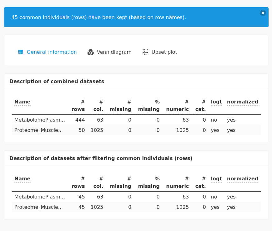
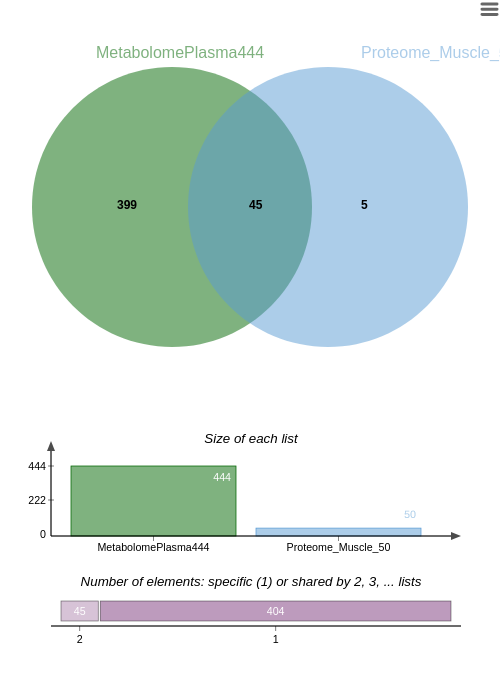
The following studies will be performed with the 45 common individuals.
17.6.2.2 Explore individuals
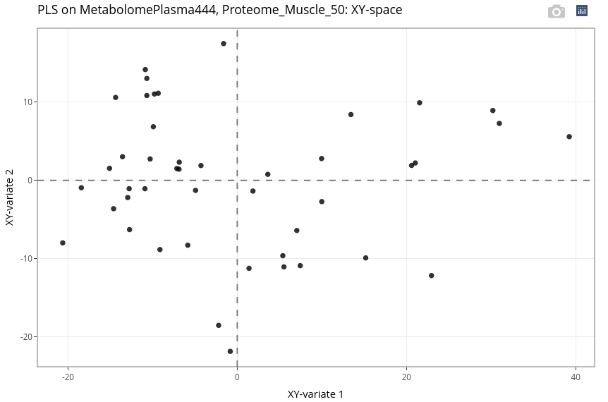
As in the previous analysis, we customize the individual plot to make the interpretation easier.
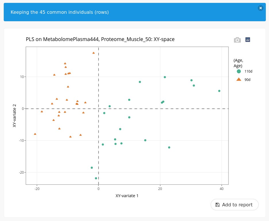
We can observe a very good differentiation between ages but in a different manner than with the two muscle omics. Here, we observe a wider heterogeneity within the piglets at day 110.
17.6.2.3 Explore variables
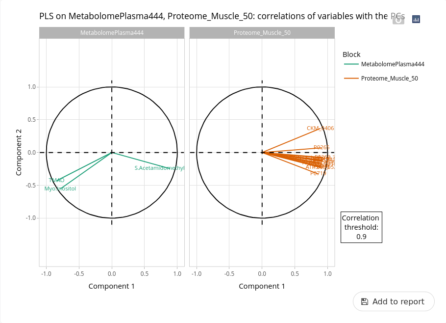
Here the two datasets contained less variables than the transcriptome. Nevertheless, we can identify variables highly correlated to the first axis and then differentiating the two ages. One of the metabolite is the myo-inositol that is known as one of the best indicator of a delayed development at the end of gestation (Lefort et al. 2020).
17.7 Multivariate supervised analysis with PLS-DA
PLS-DA is available in the Integrate panel.
17.7.1 Discrimination of the ages considering Proteome_Muscle
The supervised analysis is performed with the Proteomics_50 dataset used to explain the categorical variable Age.
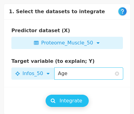
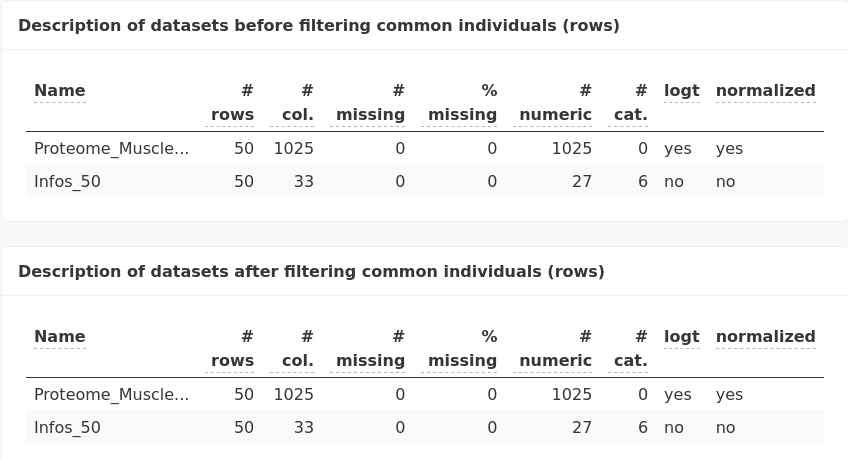
17.7.1.1 Preprocessing
The same pre-processing step is made to ensure that the analysis is performed with the same matching indivuals.
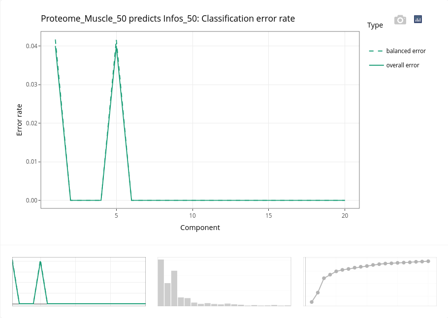
17.7.1.3 Explore individuals
In a supervised method such as PLS-DA, individuals are automatically colored according to the levels of the categorical variable.
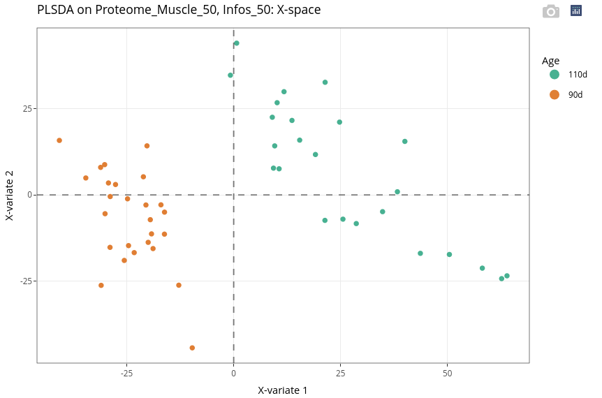
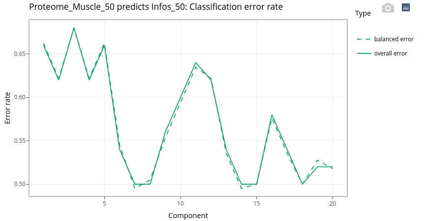
Previous results clearly indicates that the discrimination of the individuals based on their age is very easy. It is confirmed here with the very low error rate and the individual plot.
The individual plot can be modified to highlight another categorical variable and complement the interpretation of the results, for instance below with the genotype (TG_F).
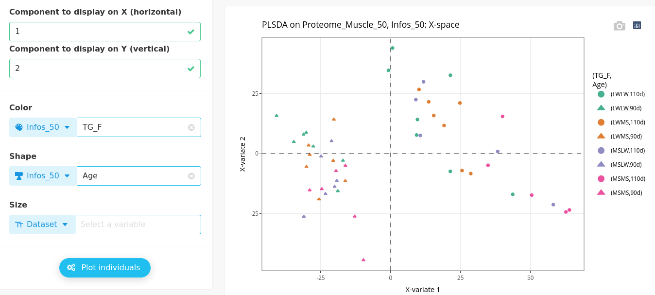
We can observe that the genotypes within each gestation age are mixed, meaning selected variables may differentiate ages whatever the genotype.
17.7.1.4 Explore variables
The interpretation of the variables has to be done using the correlation threshold.
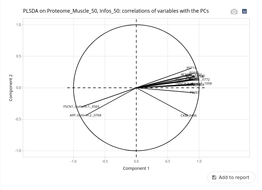
At this threshold, some variables are identified as being able to discriminate the two ages. Only two proteins (FSCN1 and AFP) are more abundant at day 90 while many others (as TNNT3) are more abundant at day 110. We can explore variation in abundance of these proteins with univariate analyses (not shown).
17.7.2 Discrimination of the genotypes considering Proteome_Muscle
With the same numerical dataset, we now intend to discriminate the individuals according to their genotype.
17.7.2.2 Explore individuals
The discrimination is not as easy as with the age. Nevertheless, the two extreme genotypes (pure breeds), MSMS (pink) and LWLW (green), are well discriminated.
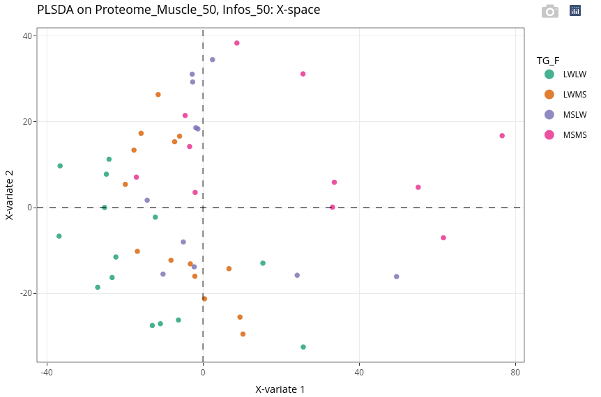
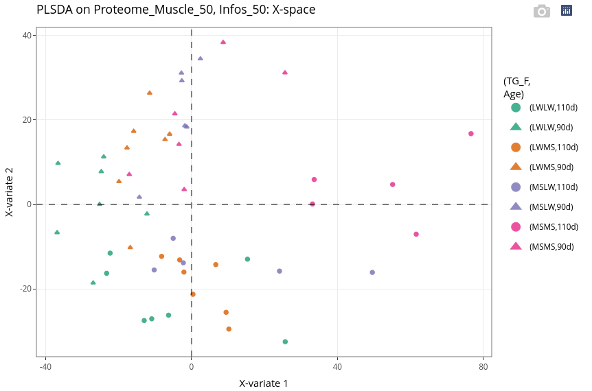
Even if the supervision is led by the genotype, we can see that the age still has a strong effect (second, vertical axis).
17.7.2.3 Explore variables
The interpretation of the variables has to be done using the correlation threshold.
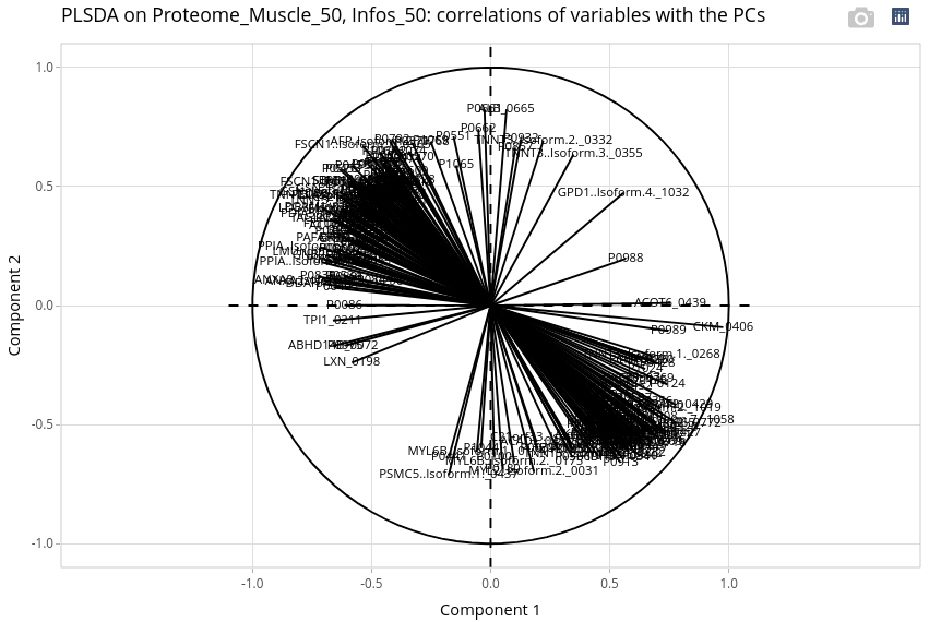
At this threshold, a lot of variables are selected. Most of them seem to be more correlated with the age effect as its effect is always very strong! Nevertheless, a protein as LXN should be more abundant in LWLW at day 90 and 110. A protein as GPD1.isoform4 should be more abundant in MSMS whatever the age. We can also explore variation in abundance of these proteins with univariate analyses (not shown).
17.7.3 Metabolome Plasma / TG_F 444 animals
Finally, the Metabolome Plasma is used to discriminate the Genotype of the 444 animals.
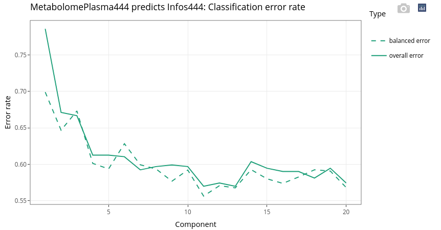
17.7.3.2 Explore individuals
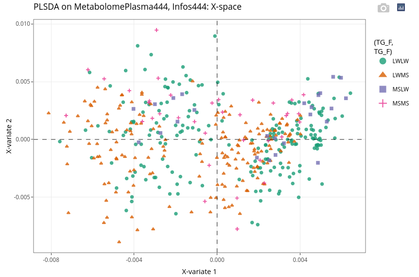
We can still observe a strong effect of the age. But within each age group, we can observe weak separation between LWLW (green, right) and LWMS (brown, left). These two genotypes groups containing many more individuals than the two other groups (see above).
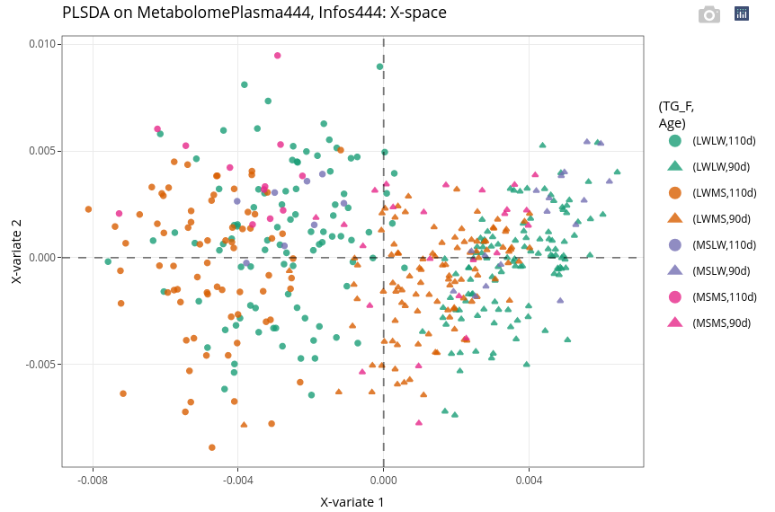
Even if the effect of the age is strong, we can observe within each age the discrimination of the two genotypes with higher number of individuals, here LWMS (in brown) and the LWLW (in green).
17.7.3.3 Explore variables
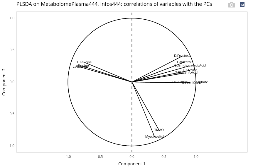
We observe 3 groups of variables. Two are very correlated to the first axis, differentiating more the ages and maybe the two genotypes LWLW and LWMS, while two variables, TMAO and myo-inositol are more correlated with the second axis. Differential analyses may explain between which conditions (age x genotype) these metabolites quantities are significantly different. A PLS between metabolites and Infos_50 may help to reveal potential correlation with some phenotypes (e.g. weight, myosine, glucose; not shown).
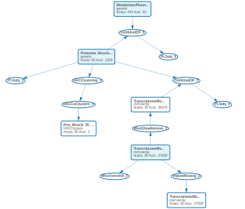
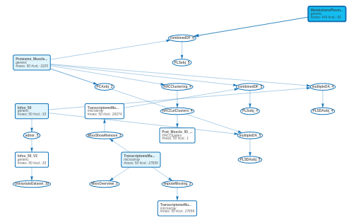
17.8 Final workflow
In conclusion, the final workflow of the case study is given below:
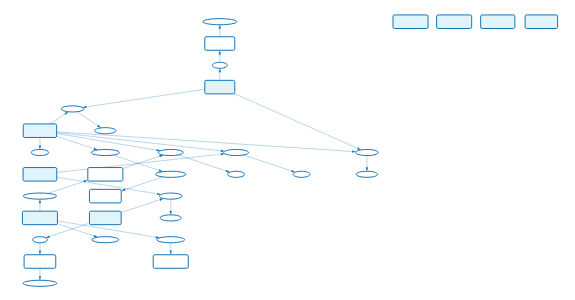
We had not analyzed four of the imported datasets. We let it to you…
17.9 Conclusion
All these analyses help to have a wide idea of the biological insight proposed by each dataset and how combination of data may increase information. We observed that age is the main factor to identify interesting variables. Transcriptome provides a huge number of variables and easily differentiates the other factors as genotype. Metabolome is more useful to explore the heterogeneity in the experiment (higher number of individuals, lower number of variables). Adding differential analyses should give statistical significance to contrasts between groups. Here, we observe that the age condition is very easy to differentiate while it is quite more difficult for the genotypes. Finally, note that some other analyses (not shown in this case studies) are also available and can be intuitively performed with ASTERICS (SOM, MFA, differential analysis, …).