Section 15 Differential Analysis

Under this menu, you can perform differential analysis to find which numeric variables of a dataset are differentially expressed between the levels of a categorical variable.

1. Parametric (ANOVA) and non-parametric (Kruskal-Wallis) tests are available and automatic choices between the two can be performed based on Shapiro-Wilk normality tests.
2. For count datasets (like RNA-seq), Binomial Negative GLM tests from edgeR are performed.
3. Post-hoc tests can be performed on variables found significant in the global test.

For further information on differential analysis on RNA-seq data:

• Robinson MD, McCarthy DJ, Smyth GK (2010). “edgeR: a Bioconductor package for differential expression analysis of digital gene expression data.” Bioinformatics, 26(1), 139-140. doi: 10.1093/bioinformatics/btp616 (Robinson, McCarthy, and Smyth 2009)

15.1 Preprocessing

Differential analysis uses two datasets: X contains numeric variables in columns (e.g., gene expression), which have to be tested, and Y contains one column (other columns can be present but will not be used) that is a categorical variable defining the conditions of the test (e.g., treatments or other information on the design of the experiment). In short, each row of Y describes the condition of the corresponding individual.
Then, differential analysis tests the equality of means for each column of X accross the groups of individuals defined by the values of Y.

Since X and Y are two different datasets (dataset1 and dataset2 below), only individuals common to X and Y are used in this analysis.

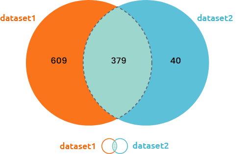
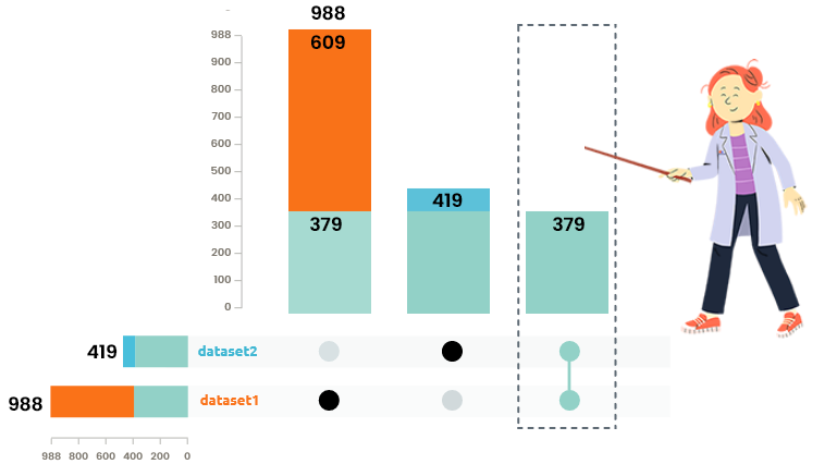
Venn diagram and upset plots are used to understand how many individuals are common / specific to each dataset. Only individuals common to all integrated datasets are used in the analysis.

15.2 Multiple tests

How to set options?
Set options to obtain results from your differential analysis:

• type can either be “parametric” (1-way ANOVA) or “nonparametric” (Kruskal-Wallis test), for standard numeric datasets. If you don’t know which one to choose, set type to “auto” and Shapiro-Wilk tests are performed to asses the normality of your data. If more than 5% of adjusted p-values (Bonferroni correction) are below 5%, type is automatically set to “nonparametric.” If your numeric dataset is a count dataset, count tests (i.e., Binomial Negative GLM tests based on edgeR implementation) are performed. It is advised to perform TMM or TMMwsp normalization before (in “Edit/Normalize dataset”), without log-transforming your data. Log-transformed datasets are processed with standard tests as explained above;

• correction is the method for multiple test adjustment: “BH” is for Benjamini-Hochberg that controls the FDR, and “Bonferroni” controls the FWER and is more stringent. You can also set that option to “none” (not advised);

• risk: is the threshold value (FDR, FWER or raw p-values) chosen to declare a result as significant.

Warning! Currently implemented tests are not well suited to deal with metagenomics data. Tests for metagenomics datasets are still to come (wait for the next release!). Meanwhile, use log-transformed counts or log-transformed compositional data to perform your differential on these datasets.

     

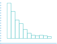
The shape of the raw p-value histogram is expected to be similar to this figure (at the left).

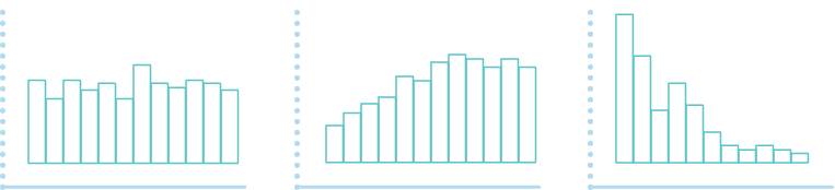
                    (a)                                                 (b)                                                 (c)

     

A flat p-value histogram (as in a) indicates that very few (or no) variables are differentially expressed. Depletion of p-values (as in b) can indicate the presence of confounding hidden variables. A p-value histogram with one or more humps (as in c) can indicate that an inappropriate statistical test was used to compute the p-values, or that the dataset has a strong correlation structure.

If your categorical variable has more than two levels and that you have significant tests, go to the “Posthoc tests” panel to further explore these tests.

15.3 Posthoc tests

15.3.1 Correction for multiple testing

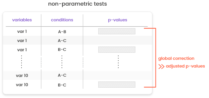
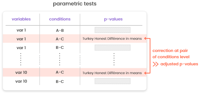
Correction for multiple testing (e.g., computation of adjusted p-values) is performed globally for non-parametric tests and tests for count data (based on edgeR). For parametric tests, the correction is performed in two tests: first, for every variable, p-values based on Tukey HDM (“honest differences in means”) are computed (and reported in column “p-values”). These p-values include a correction specific to the case where all level pairs of the same variable are tested in turns. Then, these p-values are further corrected at the condition pair level using a standard approach (Benjamini & Hochberg correction or Bonferonni correction).

15.3.2 Forest plot

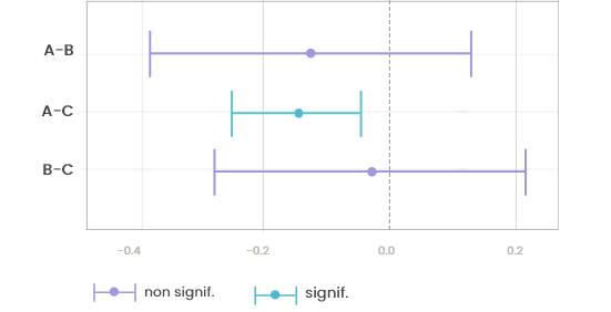
This plot is a graphical output of the post-hoc tests (tests performed on pairs of levels of the categorical variable when it has more than two levels and if the global test for 1-way ANOVA is found significant). The segments represent the confidence interval for each pairwise comparison: if 0 belongs to this interval the difference between the two means is not significant. In this plot, the correction is performed only between pairs of conditions for this variable (not accounting for all variables in the dataset).

15.4 Extract dataset

How to set options?
This screen can be used to create a new dataset in your workspace:

• with Type “extract of the original dataset,” you can extract a subset of the tested dataset containing only differential variables. When relevant, only over- or under- expressed variables can be included. In addition, for posthoc tests, variables differential for only some of the contrasts can be extracted;

• with Type “extract of the test table,” you can extract the table of results (p-values, test statistics, …) that can be further filtered by sign, variable names, contrasts, or p-value threshold (if the threshold is set to 1, all results are extracted).

You can create a new dataset that contains either the results of one of your differential analysis (table with test statistics and p-values) or a subset of your original dataset containing only variables found differentially expressed (“Sign” can also be used to select only over- or under- expressed variables). Once done, the datasets are available in “Workspace.”

     

Do not perform between sample normalization on a subset of your original variables. ASTERICS do not forbid it but it is not statistically correct.

15.5 Default parameters

Used function and default parameters:

The test type is driven by user choice or by dataset nature.

• When the test type is ‘parametric,’ the used function is summary(aov(numVar ~ catVar)) performed on all numeric variables (columns) of the input dataset, numVar, with respect to the target categorical variable, carVar,

• When the test type is ‘nonparametric,’ the used function is kruskal.test(numVar ~ catVar) performed on all numeric variables (columns) of the input dataset, numVar, with respect to the target categorical variable, carVar,

• When the test type is ‘count test,’ the used functions are edgeR::DGEList + stats::model.matrix(~ catVar) + edgeR::estimateDisp + edgeR::glmFit + edgeR::glmLRT with options norm.factors of edgeR::DGEList being the normalization factors for normalized datasets or all equal to one if the dataset has not been previously normalized, options y and design of edgeR::estimateDisp and edgeR::glmFit being the outputs of edgeR::DGEList and stats::model.matrix(~ catVar) and options glmfit and coef of glmFit being the output of edgeR::glmFit and 2:ncol(design), respectively.

• Finally, multiple test correction is performed with the function p.adjust.